Monatomic gases#

The Sackur-Tetrode equation provides a way to directly calculate the entropy of a monatomic ideal gas, based on statistical thermodynamics. It can be expressed as

\[ \overline{s} = R_{\text{univ}} \left[ \ln \left( \frac{k T}{P} \right) + \ln \left( \left[ \frac{2 \pi m k T}{h^2} \right]^{3/2} \right) + \frac{5}{2} \right] \;, \]

where

\(R_{\text{univ}}\) is the universal gas constant
\(k\) is Boltzmann’s constant
\(T\) is the temperature
\(P\) is the pressure
\(m\) is the mass of a gas particle, \(m = \frac{MW}{N_A}\)
\(N_A\) is Avogadro’s number
\(h\) is the Planck constant

To actually calculate entropy using this equation, where we want to handle units properly, we need to manipulate the equation slightly:

\[ \overline{s} = R_{\text{univ}} \left[ \ln \left( \frac{k T}{P} \left[ \frac{2 \pi m k T}{h^2} \right]^{3/2} \right) + \frac{5}{2} \right] \;, \]

We can compare this way of calculating entropy with values obtained from Cantera, which are based on the NASA thermochemical database.

import numpy as np
import cantera as ct
from scipy.constants import physical_constants

from pint import UnitRegistry
ureg = UnitRegistry()
Q_ = ureg.Quantity

# for convenience:
def to_si(quant):
    '''Converts a Pint Quantity to magnitude at base SI units.
    '''
    return quant.to_base_units().magnitude

import matplotlib.pyplot as plt
%matplotlib inline

# these are mostly for making the saved figures nicer
import matplotlib_inline.backend_inline
matplotlib_inline.backend_inline.set_matplotlib_formats('pdf', 'png')
plt.rcParams['figure.dpi']= 150
plt.rcParams['savefig.dpi'] = 150

# Obtain needed physical constants and their units

planck_constant = Q_(
   physical_constants['Planck constant'][0], 
   physical_constants['Planck constant'][1]
   )

boltzmann_constant = Q_(
    physical_constants['Boltzmann constant'][0],
    physical_constants['Boltzmann constant'][1]
    )

avogadro_number = Q_(
    physical_constants['Avogadro constant'][0],
    physical_constants['Avogadro constant'][1]
    )

gas_constant = Q_(
    physical_constants['molar gas constant'][0],
    physical_constants['molar gas constant'][1],
    )

Cantera includes the NASA thermochemical database [GM71, MGaMAR93], which contains fits for a large number of gases, including argon, helium, and monatomic oxygen.

# Extract species from NASA thermochemical database

species = ['Ar', 'He', 'O']

species_objects = {S.name: S for S in ct.Species.listFromFile('nasa_gas.cti')}
gas = ct.Solution(thermo='IdealGas', species=[species_objects[S] for S in species])

/tmp/ipykernel_5003/2360791585.py:5: DeprecationWarning: Static method 'listFromFile' is renamed to 'list_from_file'. The old name will be removed after Cantera 2.6.
  species_objects = {S.name: S for S in ct.Species.listFromFile('nasa_gas.cti')}
/tmp/ipykernel_5003/2360791585.py:5: DeprecationWarning: XML_Node::build: 
The CTI and XML input file formats are deprecated and will be removed in
Cantera 3.0. Use 'cti2yaml.py' or 'ctml2yaml.py' to convert CTI or XML input
files to the YAML format. See https://cantera.org/tutorials/legacy2yaml.html
for more information.
  species_objects = {S.name: S for S in ct.Species.listFromFile('nasa_gas.cti')}

def get_entropy(temperature, pressure, species, gas):
    """Calculates entropy of species using Sackur-Tetrode equation"""
    idx = gas.species_index(species)
    molecular_weight = Q_(gas.molecular_weights[idx], 'g/mol')
    mass = molecular_weight / avogadro_number
        
    entropy = gas_constant * (np.log(
        boltzmann_constant * temperature * (
            2 * np.pi * mass * boltzmann_constant * temperature / 
            planck_constant**2
            ) ** 1.5 / pressure
        ) + 5.0 / 2.0)
    
    return entropy

Let’s calculate the entropy of these species over the range 200–1000 K and at 1 atm, comparing the two approaches:

pressure = Q_(1, 'atm')

# range of temperatures in K
temperatures = np.linspace(200, 1000, 50) * Q_('K')

for species in gas.species():
    
    entropies = np.zeros(len(temperatures)) * Q_('J/(K*kmol)')
    entropies_ct = np.zeros(len(temperatures)) * Q_('J/(K*kmol)')
    
    for idx, temperature in enumerate(temperatures):
        gas.TPX = to_si(temperature), to_si(pressure), f'{species.name}:1.0'
        entropies_ct[idx] = Q_(gas.entropy_mole, 'J/(K*kmol)')
        
        entropies[idx] = get_entropy(temperature, pressure, species.name, gas)
    
    plt.plot(
        to_si(temperatures), entropies.to('kJ/(kmol*K)').magnitude, '-',
        color='tab:blue',
        )
    plt.plot(
        to_si(temperatures), entropies_ct.to('kJ/(kmol*K)').magnitude, 'o', 
        fillstyle='none', color='tab:blue'
        )
    
plt.xlabel('Temperature (K)')
plt.ylabel('Molar specific entropy (kJ/kmol*K)')

# text box properties
props = dict(boxstyle='round', facecolor='white', alpha=0.6)

plt.text(750, 168, 'Argon', bbox=props, ha='center', va='center')
plt.text(750, 138, 'Helium', bbox=props, ha='center', va='center')

plt.annotate(
    'Monatomic oxygen', xy=(400,170), xytext=(300,180),
    ha='center', va='center', bbox=props,
    arrowprops=dict(arrowstyle='-')
    )
plt.annotate(
    'Monatomic oxygen', xy=(400,150), xytext=(300,180),
    ha='center', va='center', bbox=props,
    arrowprops=dict(arrowstyle='-')
    )

plt.grid(True)
plt.legend([
    'Predicted by Sakur-Tetrode equation', 
    'Calculated by Cantera/NASA database'
    ])
plt.tight_layout()
plt.show()

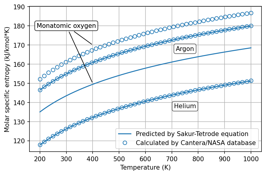
As we can see, two approaches to calculating entropy of agree nearly perfectly for helium and argon; these behave very much like ideal gases for this range of conditions.

On the other hand, monatomic oxygen (O) does not obey the ideal gas law; it exhibits strong inter-particle forces. (Oxygen normally exists as the O\(_2\) molecule, and monatomic oxygen is typically short-lived.)

Computational Thermodynamics

Monatomic gases

Monatomic gases#