Hydrogen storage tank

A hydrogen-powered vehicle is storing fuel using three onboard cylindrical tanks, each with height 65 cm and diameter 28 cm. To refuel, the tanks are connected to a reservoir of hydrogen, supplied at 300 bar and ambient temperature; a fill valve connects the reservoir to the tanks. Initially, the storage tanks have hydrogen at 60 bar and ambient temperature. The ambient temperature is 25°C.

The mass flow rate through the valve is given by

(14)\[\begin{equation} \dot{m} = C_{\text{valve}} \sqrt{ P_{\text{supply}} - P } \;, \end{equation}\]

where \(C_{\text{valve}} = 2.68 \cdot 10^{-6} \, \frac{\text{kg}}{\text{s Pa}^{0.5}}\) is the valve coefficient. The heat transfer rate from the tank walls to the hydrogen is given by

(15)\[\begin{equation} \dot{Q} = h_{\text{conv}} A_s \left( T_{\text{wall}} - T \right) \;, \end{equation}\]

where \(h_{\text{conv}} = 40 \frac{\text{W}}{\text{K m}^2}\) is the convection heat transfer coefficient.

The tanks are connected for filling for three minutes.

Problem: Determine the pressure and temperature of the hydrogen in the storage tanks as a function of time. Determine the mass of fuel added as a function of time.

import numpy as np
import cantera as ct
from scipy.integrate import solve_ivp

from pint import UnitRegistry
ureg = UnitRegistry()
Q_ = ureg.Quantity

import matplotlib.pyplot as plt
%matplotlib inline

# these are mostly for making the saved figures nicer
import matplotlib_inline.backend_inline
matplotlib_inline.backend_inline.set_matplotlib_formats('pdf', 'png')
plt.rcParams['figure.dpi']= 300
plt.rcParams['savefig.dpi'] = 300

First, let’s specify the thermodynamic states of the supply and hydrogen in the tank (initially):

temp_ambient = Q_(25, 'degC')

# supply of hydrogen has constant conditions
supply = ct.Hydrogen()
supply.TP = (
    temp_ambient.to('K').magnitude,
    Q_(300, 'bar').to('Pa').magnitude
    )

# tank properties
tank = {'number': 3, 
        'height': Q_(65, 'cm'),
        'diameter': Q_(28, 'cm')
        }

volume_tank = np.pi * tank['height'] * tank['diameter']**2 / 4.0

# initial state in the tanks, fixed by temperature and pressure
temp_initial = temp_ambient
pres_initial = Q_(60, 'bar')
hydrogen = ct.Hydrogen()
hydrogen.TP = temp_initial.to('K').magnitude, pres_initial.to('Pa').magnitude

To figure out how the system changes with time, we can do a mass balance and energy balance for the control volume. The mass balance gives

(16)\[\begin{equation} \frac{dm}{dt} = \dot{m} = C_{\text{valve}} \sqrt{ P_{\text{supply}} - P(t) } \end{equation}\]

and the energy balance gives

(17)\[\begin{equation} \dot{m} h_{\text{supply}} + \dot{Q} = \frac{dU}{dt} \;, \end{equation}\]

which provide the governing equations for how this system evolves.

We can use mass (\(m\)) and total internal energy (\(U\)) as our state variables, and construct an ODE system for these variables. We need to be able to convert between internal system properties and these:

\[\begin{split} m = \frac{ N_{\text{tank}} V_{\text{tank}} }{v} \\ U = u \, m \;. \end{split}\]

We need to define a function that evaluates the time derivative system:

def tank_rates(t, y, supply, tank, temp_ambient):
    '''Evaluates time derivatives for mass and internal energy (dm/dt and dU/dt)
    '''
    mass = Q_(y[0], 'kg')
    internal_energy = Q_(y[1], 'J')
    
    surface_area_tank = tank['number'] * (
        2 * np.pi*tank['diameter']**2 / 4.0 + 
        np.pi*tank['diameter']*tank['height']
        )
    volume_tank = np.pi * tank['height'] * tank['diameter']**2 / 4.0
    
    # specify state based on mass and internal_energy
    specific_volume = (tank['number'] * volume_tank) / mass
    specific_internal_energy = internal_energy / mass
    f = ct.Hydrogen()
    f.UV = (
        specific_internal_energy.to('J/kg').magnitude, 
        specific_volume.to('m^3/kg').magnitude
        )
    
    # evaluate dm/dt
    C_valve = Q_(2.68e-6, 'kg/(s*Pa**0.5)')
    mdot = C_valve * np.sqrt(Q_(supply.P, 'Pa') - Q_(f.P, 'Pa'))
    dmdt = mdot
    
    # evaluate dU/dt
    h_conv = Q_(40, 'W/(m**2 K)')
    Qdot = h_conv * surface_area_tank * (temp_ambient - Q_(f.T, 'K'))
    dUdt = (mdot * Q_(supply.h, 'J/kg')) + Qdot
    
    return [dmdt.to('kg/s').magnitude, dUdt.to('J/s').magnitude]

Choice of method

Here we use the 'BDF' for the method argument, which tells the solve_ivp() function to use an implicit integration method based on backward differentiation formula. Other methods are available and may be more efficient for some problems, but this is fairly accurate and can handle stiffness in the ODE system.

Finally, we can calcluate the initial mass and internal energy, then integrate over the filling time:

# initial system mass and (total) internal energy
mass_initial = (tank['number'] * volume_tank) / Q_(hydrogen.v, 'm^3/kg')
int_energy_initial = mass_initial * Q_(hydrogen.u, 'J/kg')

# Integrate over 3 minutes, 
# using backward differentiation formula (BDF) method
sol = solve_ivp(
    tank_rates, [0, 60*3], 
    [mass_initial.to('kg').magnitude, int_energy_initial.to('J').magnitude],
    args=(supply, tank, temp_ambient,),
    method='BDF'
    )

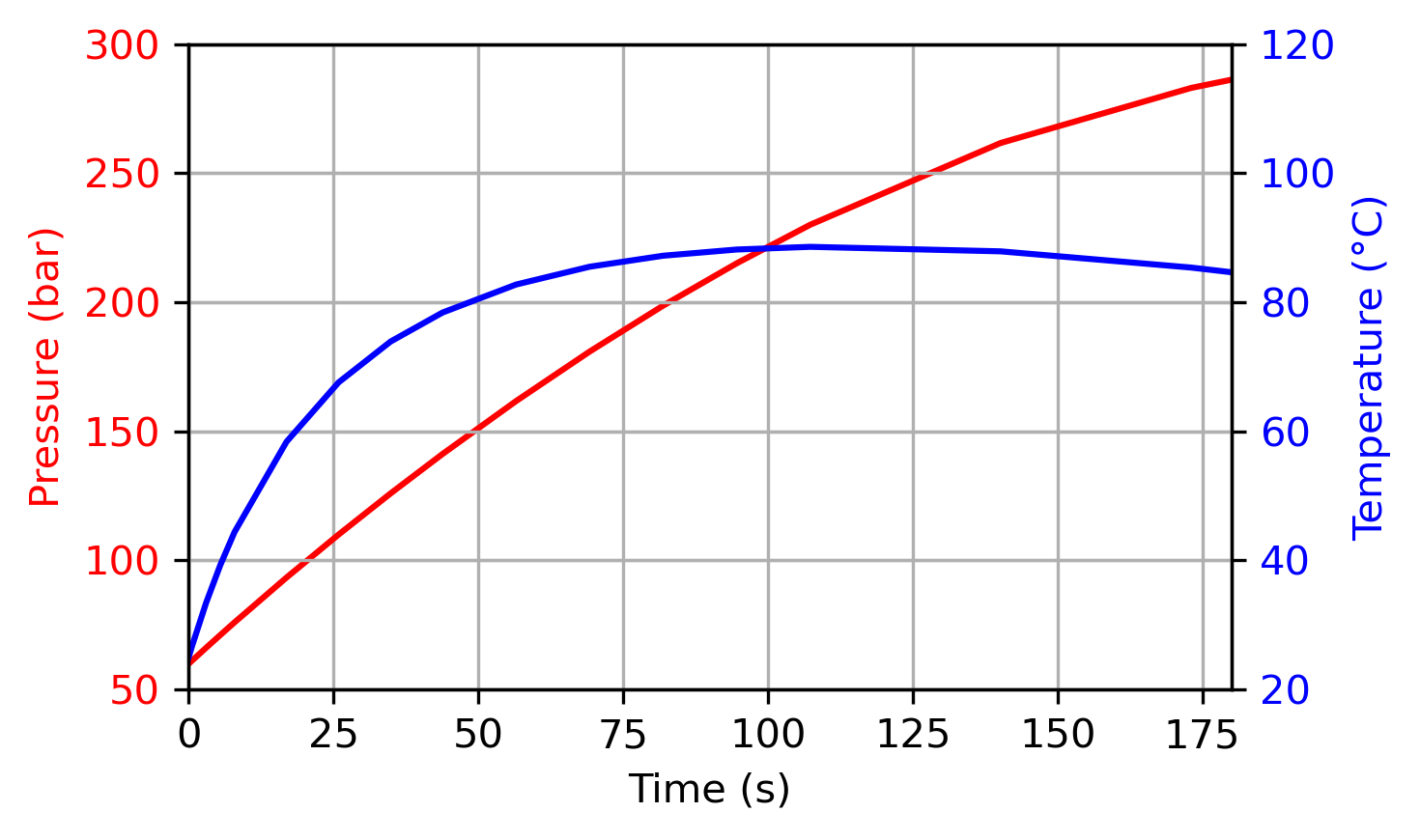
The integration was successful (it did not report an error), so now plot temperature and pressure of the tank as a function of time.

We have the system mass and internal energy as a function of time, and we’ll need to use those to specify the system at each state to obtain its properties as a function of time.

pressures = np.zeros(len(sol.y[0]))
temperatures = np.zeros(len(sol.y[0]))

for idx in range(len(sol.y[0])):
    mass = Q_(sol.y[0][idx], 'kg')
    internal_energy = Q_(sol.y[1][idx], 'J')
    
    volume_tank = np.pi * tank['height'] * tank['diameter']**2 / 4.0
    
    # calculate specific volume and specific internal energy
    # based on mass and (total) internal energys
    specific_volume = (tank['number'] * volume_tank) / mass
    specific_internal_energy = internal_energy / mass
    f = ct.Hydrogen()
    f.UV = (
        specific_internal_energy.to('J/kg').magnitude, 
        specific_volume.to('m^3/kg').magnitude
        )
    
    pressures[idx] = f.P
    temperatures[idx] = f.T
    
pressures *= ureg.Pa
temperatures *= ureg.K

fig, ax1 = plt.subplots(figsize=(5, 3))

color = 'red'
ax1.set_xlabel('Time (s)')
ax1.set_ylabel('Pressure (bar)', color=color)
ax1.plot(sol.t, pressures.to('bar').magnitude, color=color)
ax1.tick_params(axis='y', labelcolor=color)
ax1.axis([0, 180, 50, 300])
ax1.grid(True)

ax2 = ax1.twinx()  # instantiate a second axes that shares the same x-axis

color = 'blue'
# we already handled the x-label with ax1
ax2.set_ylabel('Temperature (°C)', color=color)
ax2.plot(sol.t, temperatures.to('degC').magnitude, color=color)
ax2.tick_params(axis='y', labelcolor=color)
ax2.axis([0, 180, 20, 120])
ax2.grid(True)

fig.tight_layout()  # otherwise the right y-label is slightly clipped
plt.show()

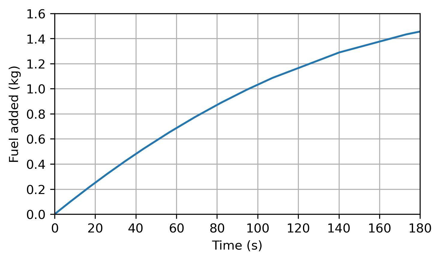
Now plot the mass of fuel added as a function of time:

mass_added = sol.y[0] - mass_initial.to('kg').magnitude
fig, ax = plt.subplots(figsize=(5, 3))
ax.plot(sol.t, mass_added)
plt.xlabel('Time (s)')
plt.axis([0, 180, 0, 1.6])
plt.ylabel('Fuel added (kg)')
plt.grid(True)
fig.tight_layout()
plt.show()