Mixture properties

Let’s consider a mixture of two gases, and evaluate how the different approaches to approximating mixture properties perform.

We have a mixture of methane (CH\(_4\)) and butane (C\(_4\)H\(_{10}\)), in a container of volume 0.241 m\(^3\). If the mixture is at 238°C, calculate the pressure. The container includes 0.18 kmol of methane and 0.474 kmol of butane.

The experimentally determined mixture pressure is 68.9 bar.

We’ll need to use CoolProp to find properties of the pure fluids (since Cantera does not currently include butane), so let’s import the necessary modules and specify the known data:

import numpy as np
from CoolProp.CoolProp import PropsSI

from pint import UnitRegistry
ureg = UnitRegistry()
Q_ = ureg.Quantity

gas_constant = Q_(PropsSI('gas_constant', 'methane'), 'J/(mol*K)')

temp = Q_(238, 'degC').to('K')
volume = Q_(0.241, 'm^3')

pres_exp = Q_(68.9, 'bar')

moles_methane = Q_(0.18, 'kmol')
moles_butane = Q_(0.274, 'kmol')

We can first evaluate the mass fractions of the components (\(x_i\)) and the molar specific volume of the mixture:

\[\begin{split} x_i = \frac{n_i}{n} \\ \bar{v} = \frac{V}{n} \end{split}\]

total_moles = moles_methane + moles_butane

x_methane = (moles_methane / total_moles).magnitude
x_butane = (moles_butane / total_moles).magnitude

specific_vol_molar = volume / total_moles
print(f'Molar specific volume: {specific_vol_molar: .3f}')

Molar specific volume: 0.531 meter ** 3 / kilomole

Ideal gas

First, we can try calculating the pressure of the mixture using the ideal gas law:

(32)\[\begin{equation} P = \frac{R T}{\bar{v}} \end{equation}\]

pres_ideal = gas_constant * temp / specific_vol_molar
print(f'Pressure (ideal gas law): {pres_ideal.to("bar"): .2f}')

Pressure (ideal gas law): 80.06 bar

Kay’s rule

Kay’s rule is the simplest mixing rule, which uses pseudo-critical properties based on values weighted by mole fractions. These are used to calculate the compressibility factor, which can in turn be used to obtain pressure:

\[\begin{split} T_c = \sum_i T_{c,i} x_i \\ P_c = \sum_i P_{c,i} x_i \\ \end{split}\]

Then, we treat the mixture as if it is a pure component with the above critical values, and obtain the reduced temperature and (molar) specific volume:

\[\begin{split} T_r = \frac{T}{T_c} \\ v_r = \frac{\bar{v} P_c}{R_u t_c} \end{split}\]

# for methane
temp_crit_methane = Q_(PropsSI('Tcrit', 'methane'), 'K')
pres_crit_methane = Q_(PropsSI('Pcrit', 'methane'), 'Pa')
molarmass_methane = Q_(PropsSI('molar_mass', 'methane'), 'kg/mol')

print('Methane critical properties: ')
print(f'T = {temp_crit_methane: .2f}, '
      f'P = {pres_crit_methane.to("bar"): .2f}'
      )

# for butane
temp_crit_butane = Q_(PropsSI('Tcrit', 'butane'), 'K')
pres_crit_butane = Q_(PropsSI('Pcrit', 'butane'), 'Pa')
molarmass_butane = Q_(PropsSI('molar_mass', 'butane'), 'kg/mol')

print('Butane critical properties: ')
print(f'T = {temp_crit_butane: .2f}, '
      f'P = {pres_crit_butane.to("bar"): .2f}'
      )

Methane critical properties: 
T = 190.56 kelvin, P = 45.99 bar
Butane critical properties: 
T = 425.12 kelvin, P = 37.96 bar

temp_crit = (
    temp_crit_methane * x_methane + 
    temp_crit_butane * x_butane
    )
pres_crit = (
    pres_crit_methane * x_methane + 
    pres_crit_butane * x_butane
    )

print(f'Pseudo critical temperature: {temp_crit: .2f}')
print(f'Pseudo critical pressure: {pres_crit.to("bar"): .2f}')

temp_red = (temp / temp_crit)
print(f'T_red = {temp_red: .2f}')

vol_red = (
    (specific_vol_molar * pres_crit) / 
    (gas_constant * temp_crit)
    ).to_base_units()
print(f'v_red = {vol_red: .3f}')

Pseudo critical temperature: 332.13 kelvin
Pseudo critical pressure: 41.14 bar
T_red = 1.54 dimensionless
v_red = 0.791 dimensionless

With the reduced temperature and specific volume, we can refer to a generalized compressibility chart (or function), which specifies the compressiblity factor as a function of reduced temperature, reduced pressure, and/or reduced specific volume for general gas mixtures. For example, see the following figures:

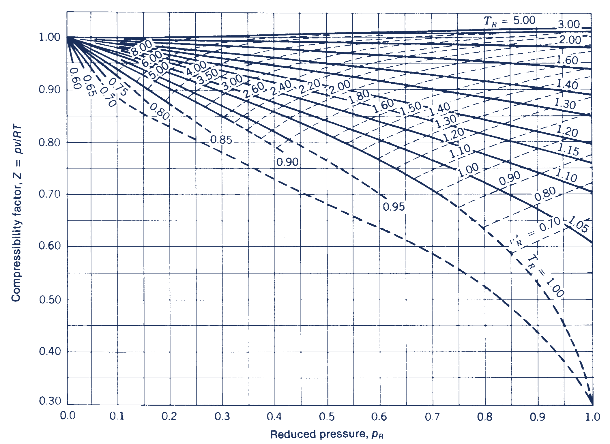
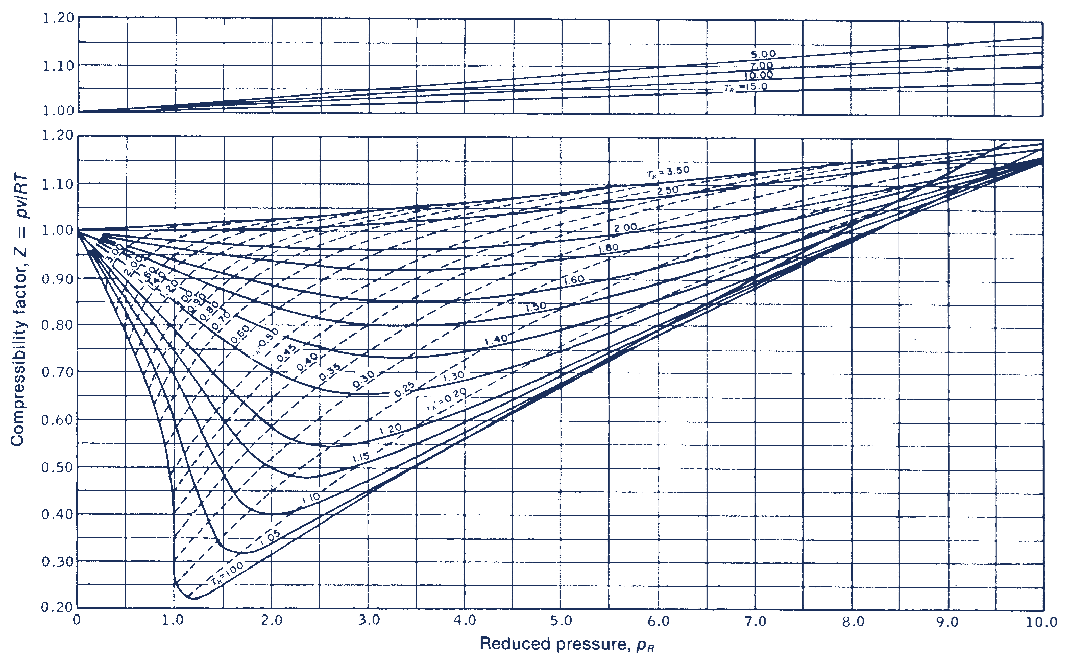
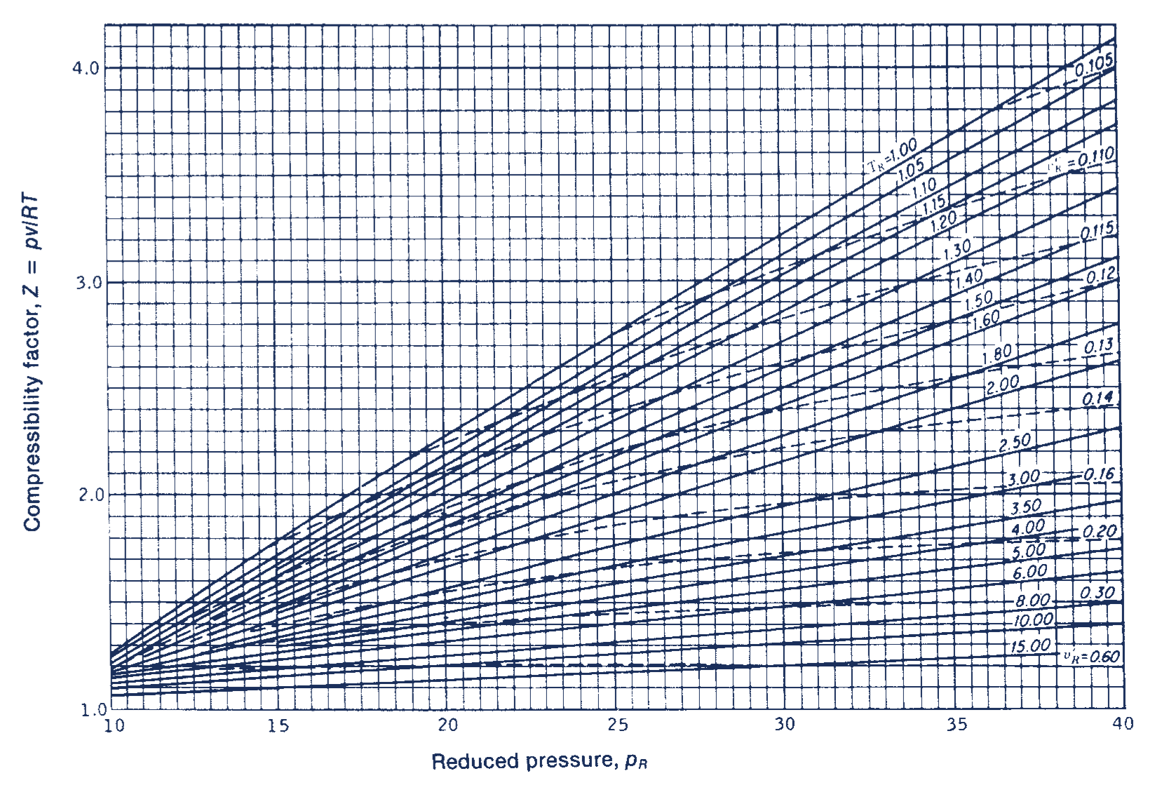
Figure: Generalized compressibility charts, for reduced pressures less than 1.0 (top), less than 10 (middle), and between 10-40 (bottom). Original source: Obert [Obe60].

If we inspect this closely and perform some visual interpolation, we can find that the compressiblity factor is approximately 0.88.

Finally, using this, we can calculate the pressure by using the relationship for compressibility factor:

(33)\[\begin{equation} P = Z \frac{R_u T}{\bar{v}} \end{equation}\]

# from chart
compress_factor = 0.88

pres_kay = (
    compress_factor * gas_constant * 
    temp / specific_vol_molar
    )
print(f"Pressure (Kay's rule): {pres_kay.to('bar'): .2f}")

Pressure (Kay's rule): 70.45 bar

van der Waals

We can obtain the coefficients \(a\) and \(b\) used in the van der Waals equation of state for the mixture by using these relations:

\[\begin{split} a = \left( \sum_{i=1} x_i \, a_i^{1/2} \right)^2 \\ b = \sum_{i=1} x_i \, b_i \;, \end{split}\]

which were proposed by Soave (1972) [Soa72].

These are then used in the equation of state

(34)\[\begin{equation} P = \frac{R_u T}{\bar{v} - b} - \frac{a}{\bar{v}^2} \end{equation}\]

# We can calculate the coefficients for each gas
# using the relations for the van der Waals equation of
# state

print('methane:')
a_methane = (
    27. * (gas_constant * temp_crit_methane)**2 /
    (64. * pres_crit_methane)
    )
b_methane = (
    gas_constant * temp_crit_methane / 
    (8. * pres_crit_methane)
    )
print(f'a = {a_methane.to("bar * (m^3/kmol)**2"): .3f}, '
      f'b = {b_methane.to("m^3/(kmol)"): .4f}'
      )

a_butane = (
    27. * (gas_constant * temp_crit_butane)**2 /
    (64. * pres_crit_butane)
    )
b_butane = (
    gas_constant * temp_crit_butane / 
    (8. * pres_crit_butane)
    )
print(f'a = {a_butane.to("bar * (m^3/kmol)**2"): .3f}, '
      f'b = {b_butane.to("m^3/(kmol)"): .4f}'
      )

methane:
a = 2.303 bar * meter ** 6 / kilomole ** 2, b = 0.0431 meter ** 3 / kilomole
a = 13.886 bar * meter ** 6 / kilomole ** 2, b = 0.1164 meter ** 3 / kilomole

a_mix = (
    x_methane * np.sqrt(a_methane) + 
    x_butane * np.sqrt(a_butane)
    )**2
b_mix = x_methane * b_methane + x_butane * b_butane

pres_vanderwaal = (
    gas_constant * temp / (specific_vol_molar - b_mix) - 
    a_mix / specific_vol_molar**2
    )
print(f'Pressure (van der Waals): {pres_vanderwaal.to("bar"): .2f}')

Pressure (van der Waals): 66.99 bar

Comparison

Now, let’s compare the accuracy of each mixture model against the experimentally observed pressure:

error_ideal = (
    100 * (pres_ideal - pres_exp) / pres_exp
    ).to_base_units()
error_kay = (
    100 * (pres_kay - pres_exp) / pres_exp
    ).to_base_units()
error_vdw = (
    100 * (pres_vanderwaal - pres_exp) / pres_exp
    ).to_base_units()

print(f'Error of ideal gas: {error_ideal.magnitude: .2f}%')
print(f'Error of Kays rule: {error_kay.magnitude: .2f}%')
print(f'Error of van der Waal mixture: {error_vdw.magnitude: .2f}%')

Error of ideal gas:  16.20%
Error of Kays rule:  2.26%
Error of van der Waal mixture: -2.78%

So, the using the ideal gas equation of state for this mixture gives a value larger than the experimental value by over 16%, while using Kay’s rule and the van der Waals equation for mixtures give values a bit under 3% above and below the experimental value.