Turbine isentropic efficiency

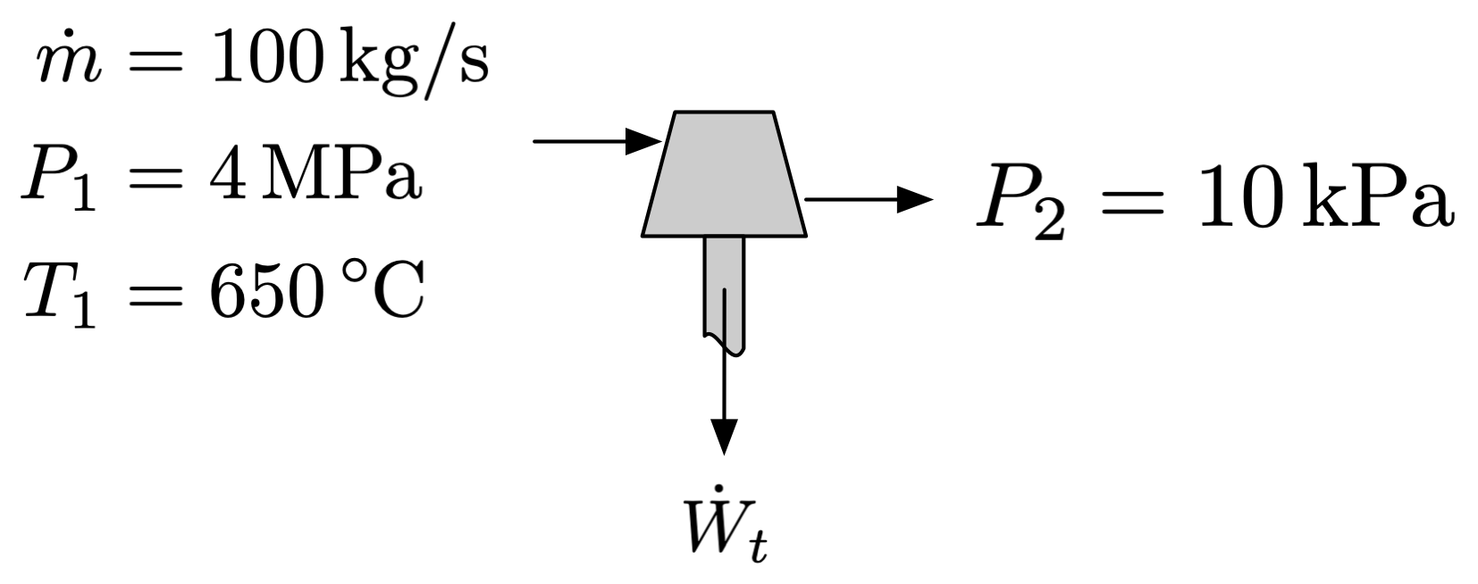
A steam turbine performs with an isentropic efficiency of \(\eta_t = 0.84\). The inlet conditions are 4 MPa and 650°C, with a mass flow rate of 100 kg/s, and the exit pressure is 10 kPa. Assume the turbine is adiabatic.

Problem:

• Determine the power produced by the turbine

• Determine the rate of entropy generation

import numpy as np
import cantera as ct

from pint import UnitRegistry
ureg = UnitRegistry()
Q_ = ureg.Quantity

We can start by specifying state 1 and the other known quantities:

temp1 = Q_(650, 'degC')
pres1 = Q_(4, 'MPa')

state1 = ct.Water()
state1.TP = temp1.to('K').magnitude, pres1.to('Pa').magnitude

mass_flow_rate = Q_(100, 'kg/s')
efficiency = 0.84

pres2 = Q_(10, 'kPa')

To apply the isentropic efficiency, we’ll need to separately consider the real turbine and an equivalent turbine operating in a reversible manner. They have the same initial conditions and mass flow rate.

For the reversible turbine, an entropy balance gives:

(21)\[\begin{equation} s_{s,2} = s_1 \end{equation}\]

and then with \(P_2\) and \(s_{s,2}\) we can fix state 2 for the reversible turbine:

state2_rev = ct.Water()
state2_rev.SP = state1.s, pres2.to('Pa').magnitude
state2_rev()

  water:

       temperature   319 K
          pressure   10000 Pa
           density   0.07464 kg/m^3
  mean mol. weight   18.016 kg/kmol
    vapor fraction   0.91292
   phase of matter   liquid-gas-mix

                          1 kg             1 kmol     
                     ---------------   ---------------
          enthalpy       -1.3594e+07       -2.4492e+08  J
   internal energy       -1.3728e+07       -2.4733e+08  J
           entropy             11017        1.9849e+05  J/K
    Gibbs function       -1.7109e+07       -3.0824e+08  J
 heat capacity c_p   inf               inf              J/K
 heat capacity c_v   nan               nan              J/K

Then, we can do an energy balance for the reversible turbine, which is also steady state and adiabatic:

\[ \dot{m} h_1 = \dot{m} h_{s,2} + \dot{W}_{s,t} \]

Then, recall that the isentropic efficiency is defined as

\[ \eta_t = \frac{\dot{W}_t}{\dot{W}_{s,t}} \;, \]

so we can obtain the actual turbine work using \(\dot{W}_t = \eta_t \dot{W}_{s,t}\) :

work_isentropic = mass_flow_rate * (
    Q_(state1.h, 'J/kg') - Q_(state2_rev.h, 'J/kg')
    )
work_actual = efficiency * work_isentropic
print(f'Actual turbine work: {work_actual.to(ureg.megawatt): .2f}')

Actual turbine work: 118.73 megawatt

Then, we can perform an energy balance on the actual turbine:

\[ \dot{m} h_1 = \dot{m} h_2 + \dot{W}_t \;, \]

which we can use with the exit pressure to fix state 2.

enthalpy2 = Q_(state1.h, 'J/kg') - (work_actual / mass_flow_rate)

state2 = ct.Water()
state2.HP = enthalpy2.to('J/kg').magnitude, pres2.to('Pa').magnitude
state2()

  water:

       temperature   328.39 K
          pressure   10000 Pa
           density   0.066165 kg/m^3
  mean mol. weight   18.016 kg/kmol
    vapor fraction   1
   phase of matter   gas

                          1 kg             1 kmol     
                     ---------------   ---------------
          enthalpy       -1.3368e+07       -2.4084e+08  J
   internal energy       -1.3519e+07       -2.4357e+08  J
           entropy             11725        2.1124e+05  J/K
    Gibbs function       -1.7219e+07       -3.1021e+08  J
 heat capacity c_p            1894.4             34129  J/K
 heat capacity c_v              1423             25637  J/K

Finally, we can perform an entropy balance on the actual turbine:

\[ \dot{m} s_1 + \dot{S}_{\text{gen}} = \dot{m} s_2 \;, \]

which allows us to find the rate of entropy generation.

entropy_gen = mass_flow_rate * (
    Q_(state2.s, 'J/(kg K)') - Q_(state1.s, 'J/(kg K)')
    )
print(f'rate of entropy generation: {entropy_gen.to("kW/K"): .2f}')

rate of entropy generation: 70.81 kilowatt / kelvin