3.3. Numerical methods for 2nd-order ODEs

We’ve gone over how to solve 1st-order ODEs using numerical methods, but what about 2nd-order or any higher-order ODEs? We can use the same methods we’ve already discussed by transforming our higher-order ODEs into a system of first-order ODEs.

Meaning, if we are given a 2nd-order ODE

(3.53)\[\begin{equation} \frac{d^2 y}{dx^2} = y^{\prime\prime} = f(x, y, y^{\prime}) \end{equation}\]

we can transform this into a system of two 1st-order ODEs that are coupled:

(3.54)\[\begin{align} \frac{dy}{dx} &= y^{\prime} = u \\ \frac{du}{dx} &= u^{\prime} = y^{\prime\prime} = f(x, y, u) \end{align}\]

where \(f(x, y, u)\) is the same as that given above for \(\frac{d^2 y}{dx^2}\).

Thus, instead of a 2nd-order ODE to solve, we have two 1st-order ODEs:

(3.55)\[\begin{align} y^{\prime} &= u \\ u^{\prime} &= f(x, y, u) \end{align}\]

So, we can use all of the methods we have talked about so far to solve 2nd-order ODEs by transforming the one equation into a system of two 1st-order equations.

3.3.1. Higher-order ODEs

This works for higher-order ODEs too! For example, if we have a 3rd-order ODE, we can transform it into a system of three 1st-order ODEs:

(3.56)\[\begin{align} \frac{d^3 y}{dx^3} &= f(x, y, y^{\prime}, y^{\prime\prime}) \\ \rightarrow y^{\prime} &= u \\ u^{\prime} &= y^{\prime\prime} = w \\ w^{\prime} &= y^{\prime\prime\prime} = f(x, y, u, w) \end{align}\]

# import libraries for numerical functions and plotting
import numpy as np
import matplotlib.pyplot as plt

# these lines are only for helping improve the display
import matplotlib_inline.backend_inline
matplotlib_inline.backend_inline.set_matplotlib_formats('pdf', 'png')
plt.rcParams['figure.dpi']= 300
plt.rcParams['savefig.dpi'] = 300

3.3.2. Example: mass-spring problem

For example, let’s solve a forced damped mass-spring problem given by a 2nd-order ODE:

(3.57)\[\begin{equation} y^{\prime\prime} + 5y^{\prime} + 6y = 10 \sin \omega t \end{equation}\]

with the initial conditions \(y(0) = 0\) and \(y^{\prime}(0) = 5\).

We start by transforming the equation into two 1st-order ODEs. Let’s use the variables \(z_1 = y\) and \(z_2 = y^{\prime}\):

(3.58)\[\begin{align} \frac{dz_1}{dt} &= z_1^{\prime} = z_2 \\ \frac{dz_2}{dt} &= z_2^{\prime} = y^{\prime\prime} = 10 \sin \omega t - 5z_2 - 6z_1 \end{align}\]

3.3.2.1. Forward Euler

Then, let’s solve numerically using the forward Euler method. Recall that the recursion formula for forward Euler is:

(3.59)\[\begin{equation} y_{i+1} = y_i + \Delta x f(x_i, y_i) \end{equation}\]

where \(f(x,y) = \frac{dy}{dx}\).

Let’s solve using \(\omega = 1\) and with a step size of \(\Delta t = 0.1\), over \(0 \leq t \leq 3\).

We can compare this against the exact solution, obtainable using the method of undetermined coefficients:

(3.60)\[\begin{equation} y(t) = -6 e^{-3t} + 7 e^{-2t} + \sin t - \cos t \end{equation}\]

# plot exact solution first
time = np.linspace(0, 3)
y_exact = (
    -6*np.exp(-3*time) + 7*np.exp(-2*time) + 
    np.sin(time) - np.cos(time)
    )
plt.plot(time, y_exact, label='Exact')

omega = 1

dt = 0.1
time = np.arange(0, 3.001, dt)

f = lambda t,z1,z2: 10*np.sin(omega*t) - 5*z2 - 6*z1

z1 = np.zeros_like(time)
z2 = np.zeros_like(time)
# initial conditions
z1[0] = 0
z2[0] = 5

# Forward Euler iterations
for idx, t in enumerate(time[:-1]):
    z1[idx+1] = z1[idx] + dt*z2[idx]
    z2[idx+1] = z2[idx] + dt*f(t, z1[idx], z2[idx])

plt.plot(time, z1, 'o--', label='Forward Euler solution')
plt.xlabel('time')
plt.ylabel('displacement')
plt.legend()
plt.grid(True)
plt.show()

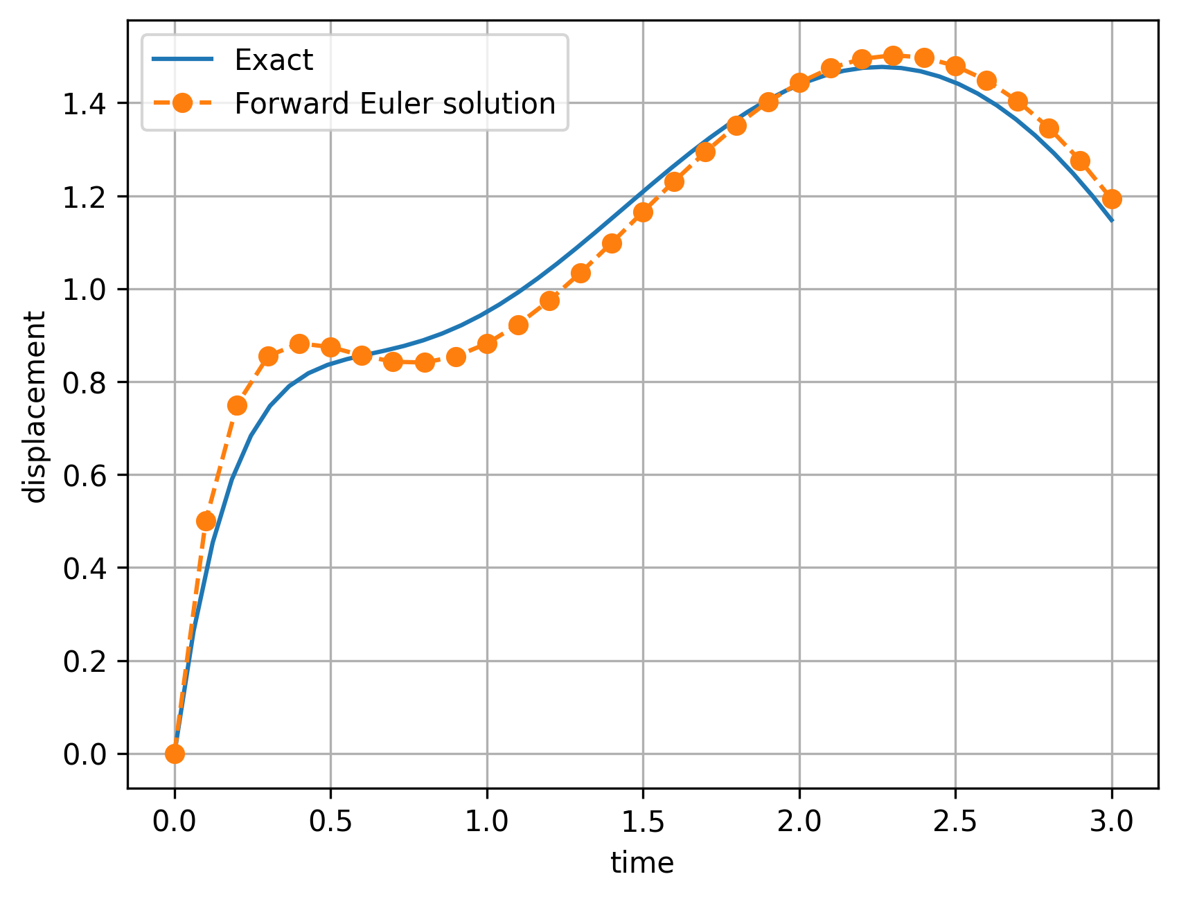
Since the method is only first-order accurate, we see both qualitative and quantiative differences compared with the exact solution, but the overall solution agrees. We can use more-accurate methods to better-capture the exact solution.

3.3.2.2. Heun’s Method

For schemes that involve more than one stage, like Heun’s method, we’ll need to implement both stages for each 1st-order ODE. For example:

# plot exact solution first
time = np.linspace(0, 3)
y_exact = (
    -6*np.exp(-3*time) + 7*np.exp(-2*time) + 
    np.sin(time) - np.cos(time)
    )
plt.plot(time, y_exact, label='Exact')

omega = 1

dt = 0.1
time = np.arange(0, 3.001, dt)

f = lambda t,z1,z2: 10*np.sin(omega*t) - 5*z2 - 6*z1

z1 = np.zeros_like(time)
z2 = np.zeros_like(time)
# initial conditions
z1[0] = 0
z2[0] = 5

# Forward Euler iterations
for idx, t in enumerate(time[:-1]):
    # predictor
    z1p = z1[idx] + dt*z2[idx]
    z2p = z2[idx] + dt*f(t, z1[idx], z2[idx])
    
    # corrector
    z1[idx+1] = z1[idx] + 0.5*dt*(z2[idx] + z2p)
    z2[idx+1] = z2[idx] + 0.5*dt*(
        f(t, z1[idx], z2[idx]) + f(time[idx+1], z1p, z2p)
        )

plt.plot(time, z1, 'o--', label='Heuns method solution')
plt.xlabel('time')
plt.ylabel('displacement')
plt.legend()
plt.grid(True)
plt.show()

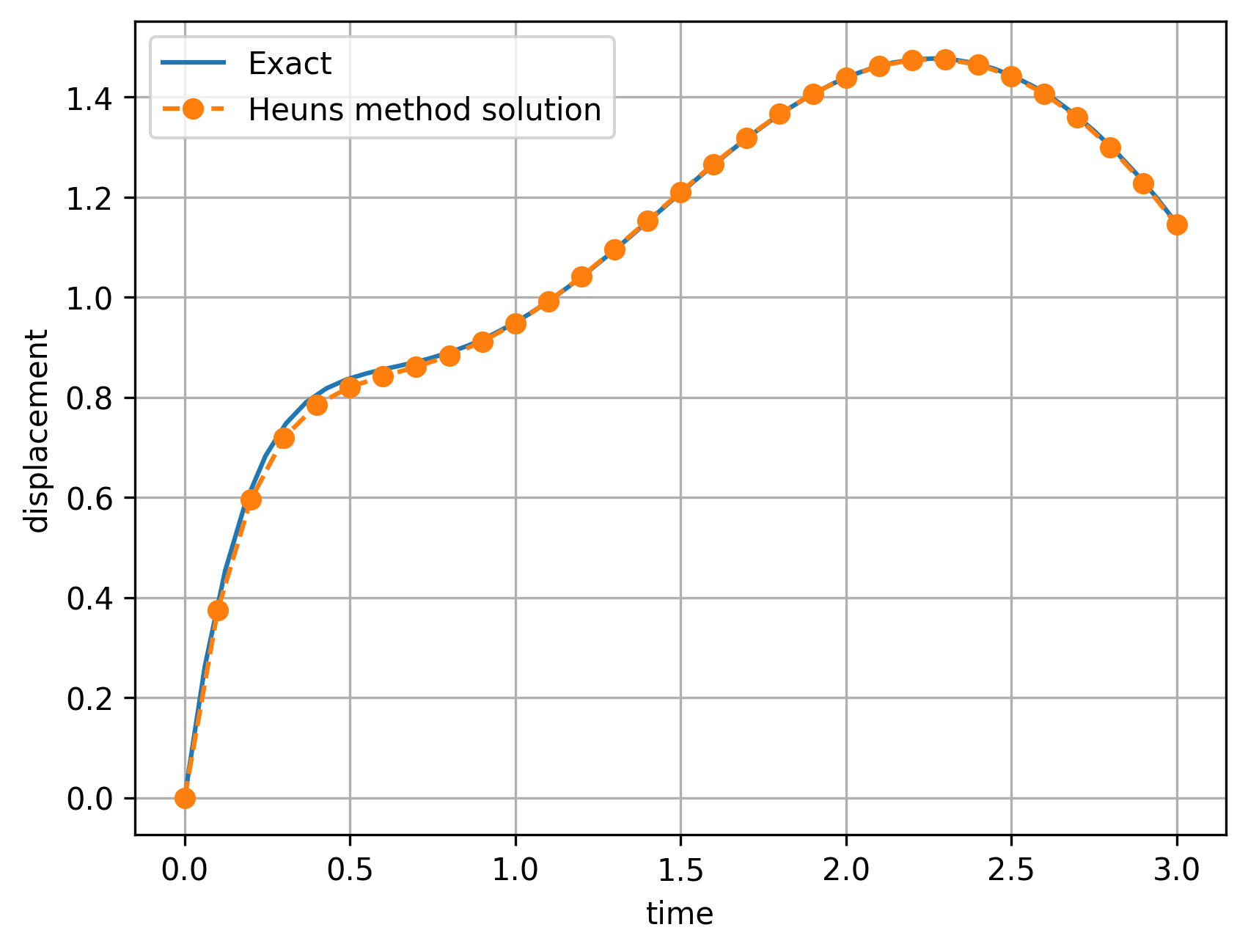
As expected, the numerical solution using Heun’s method agrees much more closely to the exact solution (vs. forward Euler), though we can still see some error due to the relatively large step size.

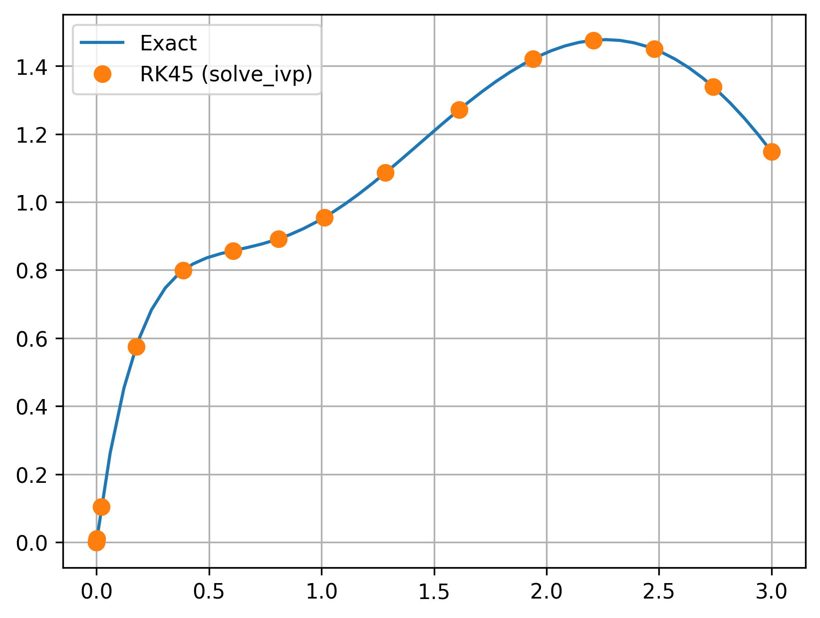
3.3.2.3. Runge-Kutta method

We can also solve using the 4th-order Runge–Kutta method available through the solve_ivp() function, by providing a function that defines the system of first-order ODEs.

Since there are technically two variables being integrated (\(z_1\) representing \(y\), and \(z_2\) representing \(y^{\prime}\)), the solution object contained in sol.y will be a two-dimensional array.

The first column, sol.y[0,:], will contain \(y\) and the second column, sol.y[1,;], will contain \(y^{\prime}\). We are typically mostly interested in the solution to \(y\).

from scipy.integrate import solve_ivp

# plot exact solution first
time = np.linspace(0, 3)
y_exact = (
    -6*np.exp(-3*time) + 7*np.exp(-2*time) + 
    np.sin(time) - np.cos(time)
    )
plt.plot(time, y_exact, label='Exact')

def mass_spring(time, z):
    '''Function providing dz/dt derivative system'''
    omega = 1    
    return [z[1], 10*np.sin(omega*time) - 6*z[0] - 5*z[1]]

sol = solve_ivp(mass_spring, [0, 3], [0, 5], method='RK45')

plt.plot(
    sol.t, sol.y[0,:], '.', 
    markersize=15, label='RK45 (solve_ivp)'
    )
plt.grid(True)
plt.legend()
plt.show()

3.3.3. Backward Euler for 2nd-order ODEs

We saw how to implement the Backward Euler method for a 1st-order ODE, but what about a 2nd-order ODE? (Or in general a system of 1st-order ODEs?)

The recursion formula is the same, except now our dependent variable is an array/vector:

(3.61)\[\begin{equation} \mathbf{y}_{i+1} = \mathbf{y}_i + \Delta t \, \mathbf{f} \left( t_{i+1} , \mathbf{y}_{i+1} \right) \end{equation}\]

where the bolded \(\mathbf{y}\) and \(\mathbf{f}\) indicate array quantities (in other words, they hold more than one value).

In general, we can use Backward Euler to solve 2nd-order ODEs in a similar fashion as our other numerical methods:

1. Convert the 2nd-order ODE into a system of two 1st-order ODEs

2. Insert the ODEs into the Backward Euler recursion formula and solve for \(\mathbf{y}_{i+1}\)

The main difference is that we will now have a system of two equations and two unknowns: \(y_{1, i+1}\) and \(y_{2, i+1}\).

Let’s demonstrate with an example:

(3.62)\[\begin{equation} y^{\prime\prime} + 6 y^{\prime} + 5y = 10 \quad y(0) = 0 \quad y^{\prime}(0) = 5 \end{equation}\]

where the exact solution is

(3.63)\[\begin{equation} y(t) = -\frac{3}{4} e^{-5t} - \frac{5}{4} e^{-t} + 2 \end{equation}\]

To solve numerically,

1. Convert the 2nd-order ODE into a system of two 1st-order ODEs:

(3.64)\[\begin{gather} y_1 = y \quad y_1(t=0) = 0 \\ y_2 = y^{\prime} \quad y_2 (t=0) = 5 \end{gather}\]

Then, for the derivatives of these variables:

(3.65)\[\begin{align} y_1^{\prime} &= y_2 \\ y_2^{\prime} &= 10 - 6 y_2 - 5 y_1 \end{align}\]

2. Then plug these derivatives into the Backward Euler recursion formulas and solve for \(y_{1,i+1}\) and \(y_{2,i+1}\):

(3.66)\[\begin{align} y_{1, i+1} &= y_{1, i} + \Delta t \, y_{2,i+1} \\ y_{2, i+1} &= y_{2, i} + \Delta t \left( 10 - 6 y_{2, i+1} - 5 y_{1,i+1} \right) \\ \rightarrow y_{1, i+1} - \Delta t \, y_{2, i+1} &= y_{1,i} \\ 5 \Delta t \, y_{1, i+1} + (1 + 6 \Delta t) y_{2, i+1} &= y_{2,i} + 10 \Delta t \end{align}\]

or, represented as a product of a coefficient matrix and a vector:

(3.67)\[\begin{align} \begin{bmatrix} 1 & -\Delta t \\ 5 \Delta t & (1+6\Delta t)\end{bmatrix} \begin{bmatrix} y_{1, i+1} \\ y_{2, i+1} \end{bmatrix} &= \begin{bmatrix} y_{1,i} \\ y_{2,i} + 10 \Delta t \\ \end{bmatrix} \\ \mathbf{A} \mathbf{y}_{i+1} &= \mathbf{b} \end{align}\]

To isolate \(\mathbf{y}_{i+1}\) and get a usable recursion formula, we need to solve this system of two equations. We could solve this by hand using the substitution method, or we can use Cramer’s rule:

(3.68)\[\begin{align} y_{1, i+1} &= \frac{ y_{1,i} (1 + 6 \Delta t) + \Delta t \left( y_{2,i} + 10 \Delta t \right)}{1 + 6 \Delta t + 5 \Delta t^2} \\ y_{2, i+1} &= \frac{ y_{2,i} + 10 \Delta t - 5 \Delta t y_{1,i}}{1 + 6 \Delta t + 5 \Delta t^2} \end{align}\]

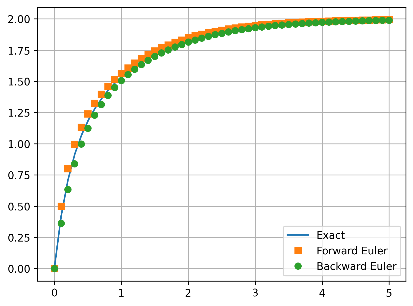
Let’s confirm that this gives us a good, well-behaved numerical solution and compare with the Forward Euler method:

# Exact solution
time = np.linspace(0, 5)
y_exact = lambda t: -0.75*np.exp(-5*t) - 1.25*np.exp(-t) + 2
plt.plot(time, y_exact(time), label='Exact')

dt = 0.1
time = np.arange(0, 5.001, dt)

# Forward Euler
f = lambda t,y1,y2: 10 - 6*y2 - 5*y1
y1 = np.zeros_like(time)
y2 = np.zeros_like(time)
y1[0] = 0
y2[0] = 5
for idx, t in enumerate(time[:-1]):
    y1[idx+1] = y1[idx] + dt*y2[idx]
    y2[idx+1] = y2[idx] + dt*f(t, y1[idx], y2[idx])

plt.plot(time, y1, 's', label='Forward Euler')

# Backward Euler
# use a single array to contain both variables being integrated
y_vals = np.zeros((len(time), 2))
y_vals[0,0] = 0
y_vals[0,1] = 5
for idx, t in enumerate(time[:-1]):
    denom = 1 + 6*dt + 5*dt**2
    y_vals[idx+1,0] = (
        y_vals[idx,0]*(1 + 6*dt) + dt*(y_vals[idx,1] + 10*dt)
        ) / denom
    y_vals[idx+1,1] = (
        y_vals[idx,1] + 10*dt - y_vals[idx,0]*5*dt
        ) / denom

plt.plot(time, y_vals[:,0], 'o', label='Backward Euler')
plt.legend()
plt.grid(True)
plt.show()

print(
    'Maximum error of Forward Euler: '
    f'{np.max(np.abs(y1 - y_exact(time))): .3f}'
    )
print(
    'Maximum error of Forward Euler: '
    f'{np.max(np.abs(y_vals[:,0] - y_exact(time))): .3f}'
    )

Maximum error of Forward Euler:  0.099
Maximum error of Forward Euler:  0.068

So, for \(\Delta t = 0.1\), we see that the Forward and Backward Euler methods give an error \(\mathcal{O}(\Delta t)\), as expected since both methods are first-order accurate.

Let’s see how they compare for a larger step size:

# Exact solution
time = np.linspace(0, 5)
y_exact = lambda t: -0.75*np.exp(-5*t) - 1.25*np.exp(-t) + 2
plt.plot(time, y_exact(time), label='Exact')

dt = 0.5
time = np.arange(0, 5.001, dt)

# Forward Euler
f = lambda t,y1,y2: 10 - 6*y2 - 5*y1
y1 = np.zeros_like(time)
y2 = np.zeros_like(time)
y1[0] = 0
y2[0] = 5
for idx, t in enumerate(time[:-1]):
    y1[idx+1] = y1[idx] + dt*y2[idx]
    y2[idx+1] = y2[idx] + dt*f(t, y1[idx], y2[idx])

plt.plot(time, y1, 's', label='Forward Euler')

# Backward Euler
# use a single array to contain both variables being integrated
y_vals = np.zeros((len(time), 2))
y_vals[0,0] = 0
y_vals[0,1] = 5
for idx, t in enumerate(time[:-1]):
    denom = 1 + 6*dt + 5*dt**2
    y_vals[idx+1,0] = (
        y_vals[idx,0]*(1 + 6*dt) + dt*(y_vals[idx,1] + 10*dt)
        ) / denom
    y_vals[idx+1,1] = (
        y_vals[idx,1] + 10*dt - y_vals[idx,0]*5*dt
        ) / denom

plt.plot(time, y_vals[:,0], 'o', label='Backward Euler')
plt.legend()
plt.grid(True)
plt.show()

print(
    'Maximum error of Forward Euler: '
    f'{np.max(np.abs(y1 - y_exact(time))): .3f}'
    )
print(
    'Maximum error of Backward Euler: '
    f'{np.max(np.abs(y_vals[:,0] - y_exact(time))): .3f}'
    )

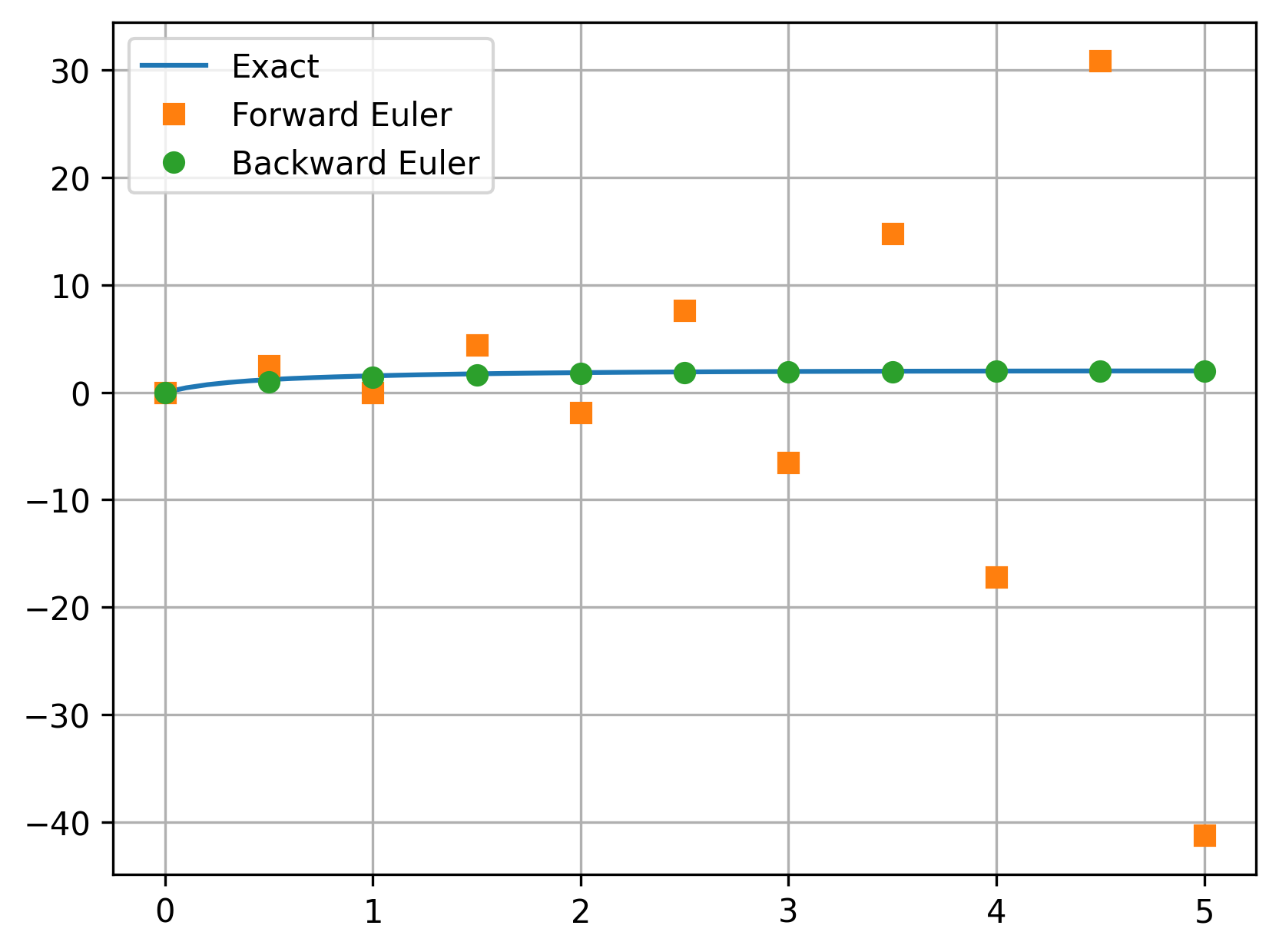
Maximum error of Forward Euler:  43.242
Maximum error of Backward Euler:  0.228

Backward Euler, since it is unconditionally stable, remains well-behaved at this larger step size, while the Forward Euler method blows up.

One other thing: instead of using Cramer’s rule to get expressions for \(y_{1,i+1}\) and \(y_{2,i+1}\), we could instead use built-in linear algebra routines to solve the linear system of equations at each time step, using the function np.linalg.solve().

To do that, we could replace it with

A = np.array([1,  -dt], [5*dt, 1+6*dt])
b = np.array([y_vals[idx,0], y_vals[idx,1]+10*dt])
y_vals[idx+1,:] = np.linalg.solve(A, b)

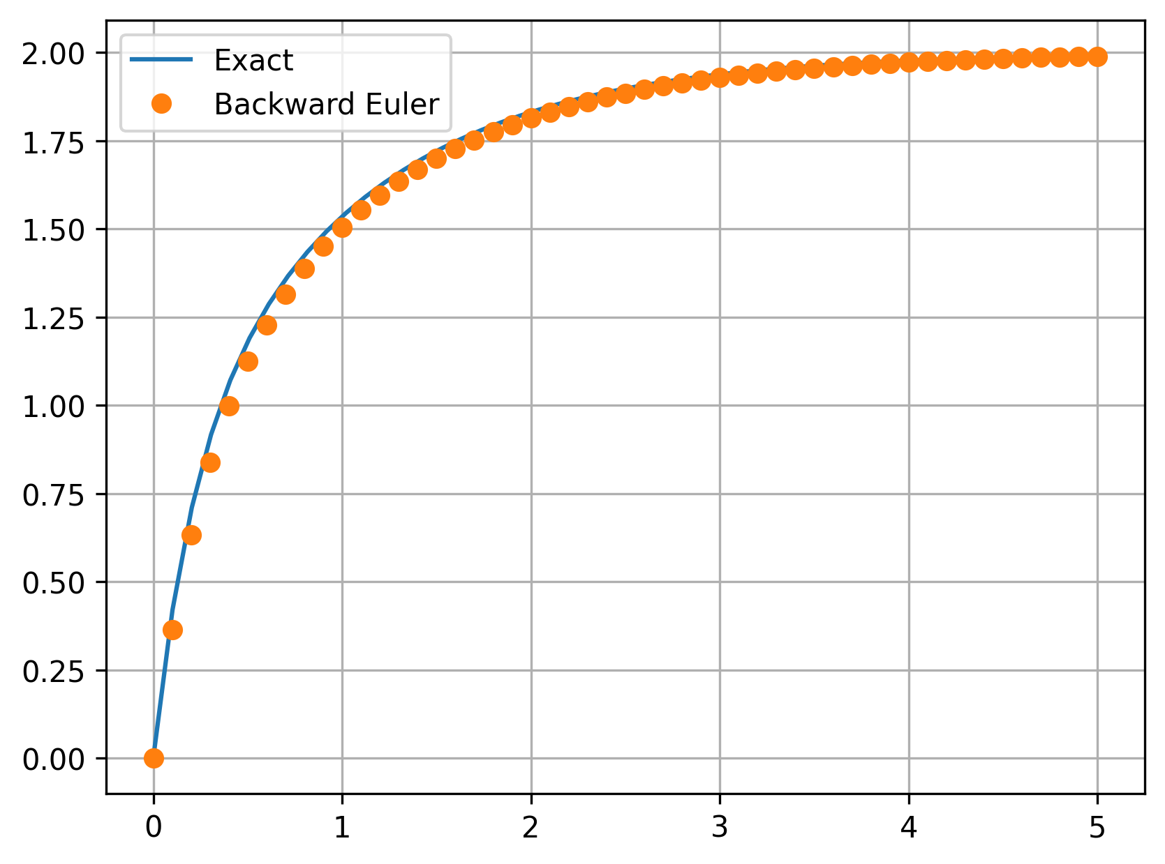
Let’s confirm that this gives the same answer:

# Exact solution
time = np.linspace(0, 5)
y_exact = lambda t: -0.75*np.exp(-5*t) - 1.25*np.exp(-t) + 2
plt.plot(time, y_exact(time), label='Exact')

dt = 0.1
time = np.arange(0, 5.001, dt)

# Backward Euler
y_vals = np.zeros((len(time), 2))
y_vals[0,0] = 0
y_vals[0,1] = 5
for idx, t in enumerate(time[:-1]):
    A = np.array([[1,  -dt], [5*dt, 1+6*dt]])
    b = np.array([y_vals[idx,0], y_vals[idx,1]+10*dt])
    y_vals[idx+1,:] = np.linalg.solve(A, b)

plt.plot(time, y_vals[:,0], 'o', label='Backward Euler')
plt.legend()
plt.grid(True)
plt.show()

3.3.4. Cramer’s Rule

Cramer’s Rule provides a solution method for a system of linear equations, where the number of equations equals the number of unknowns. It works for any number of equations/unknowns, but isn’t really practical for more than two or three. We’ll focus on using it for a system of two equations, with two unknowns \(x_1\) and \(x_2\):

(3.69)\[\begin{gather} a_{11} x_1 + a_{12} x_2 = b_1 \\ a_{21} x_1 + a_{22} x_2 = b_2 \\ \text{or } \mathbf{A} \mathbf{x} = \mathbf{b} \end{gather}\]

where

(3.70)\[\begin{gather} \mathbf{A} = \begin{bmatrix} a_{11} & a_{12} \\ a_{21} & a_{22} \end{bmatrix} \\ \mathbf{x} = \begin{bmatrix} x_1 \\ x_2 \end{bmatrix} \\ \mathbf{b} = \begin{bmatrix} b_1 \\ b_2 \end{bmatrix} \end{gather}\]

The solutions for the unknowns are then

(3.71)\[\begin{align} x_1 &= \frac{ \begin{vmatrix} b_1 & a_{12} \\ b_2 & a_{22} \end{vmatrix} }{D} = \frac{b_1 a_{22} - a_{12} b_2}{D} \\ x_2 &= \frac{ \begin{vmatrix} a_{11} & b_1 \\ a_{21} & b_2 \end{vmatrix} }{D} = \frac{a_{11} b_2 - b_1 a_{21}}{D} \end{align}\]

where \(D\) is the determinant of \(\mathbf{A}\):

(3.72)\[\begin{equation} D = \det(\mathbf{A}) = \begin{vmatrix} a_{11} & a_{12} \\ a_{21} & a_{22} \end{vmatrix} = a_{11} a_{22} - a_{12} a_{21} \end{equation}\]

This works as long as the determinant does not equal zero.