5.2. Parabolic PDEs

# import libraries for numerical functions and plotting
import numpy as np
import matplotlib.pyplot as plt

# these lines are only for helping improve the display
import matplotlib_inline.backend_inline
matplotlib_inline.backend_inline.set_matplotlib_formats('pdf', 'png')
plt.rcParams['figure.dpi']= 300
plt.rcParams['savefig.dpi'] = 300

A classic example of a parabolic partial differential equation (PDE) is the one-dimensional unsteady heat equation:

(5.25)\[\begin{equation} \frac{\partial T}{\partial t} = \alpha \frac{\partial^2 T}{\partial t^2} \end{equation}\]

where \(T(x,t)\) is the temperature varying in space and time, and \(\alpha\) is the thermal diffusivity: \(\alpha = k / (\rho c_p)\), which is a constant.

We can solve this using finite differences to represent the spatial derivatives and time derivatives separately. First, let’s rearrange the PDE slightly:

(5.26)\[\begin{equation} \frac{\partial^2 T}{\partial x^2} = \frac{1}{\alpha} \frac{\partial T}{\partial t} \end{equation}\]

5.2.1. Explicit scheme

Let’s use a central difference for the spatial derivative with a spacing of \(\Delta x\), and a forward difference for the time derivative with a time-step size of \(\Delta t\). With these choices, we can obtain an approximation to the PDE that applies at time \(t^k\) and spatial location \(x_i\):

(5.27)\[\begin{equation} \frac{T_{i-1}^k - 2 T_i^k + T_{i+1}^k}{\Delta x^2} = \frac{1}{\alpha} \left( \frac{T_i^{k+1} - T_i^k}{\Delta t} \right) \end{equation}\]

where \(T_i^k\) is the temperature at time \(t^k\) and spatial location \(x_i\). The following figure shows the stencil of points involved in the PDE applied to location \(x_i\) at time \(t^k\).

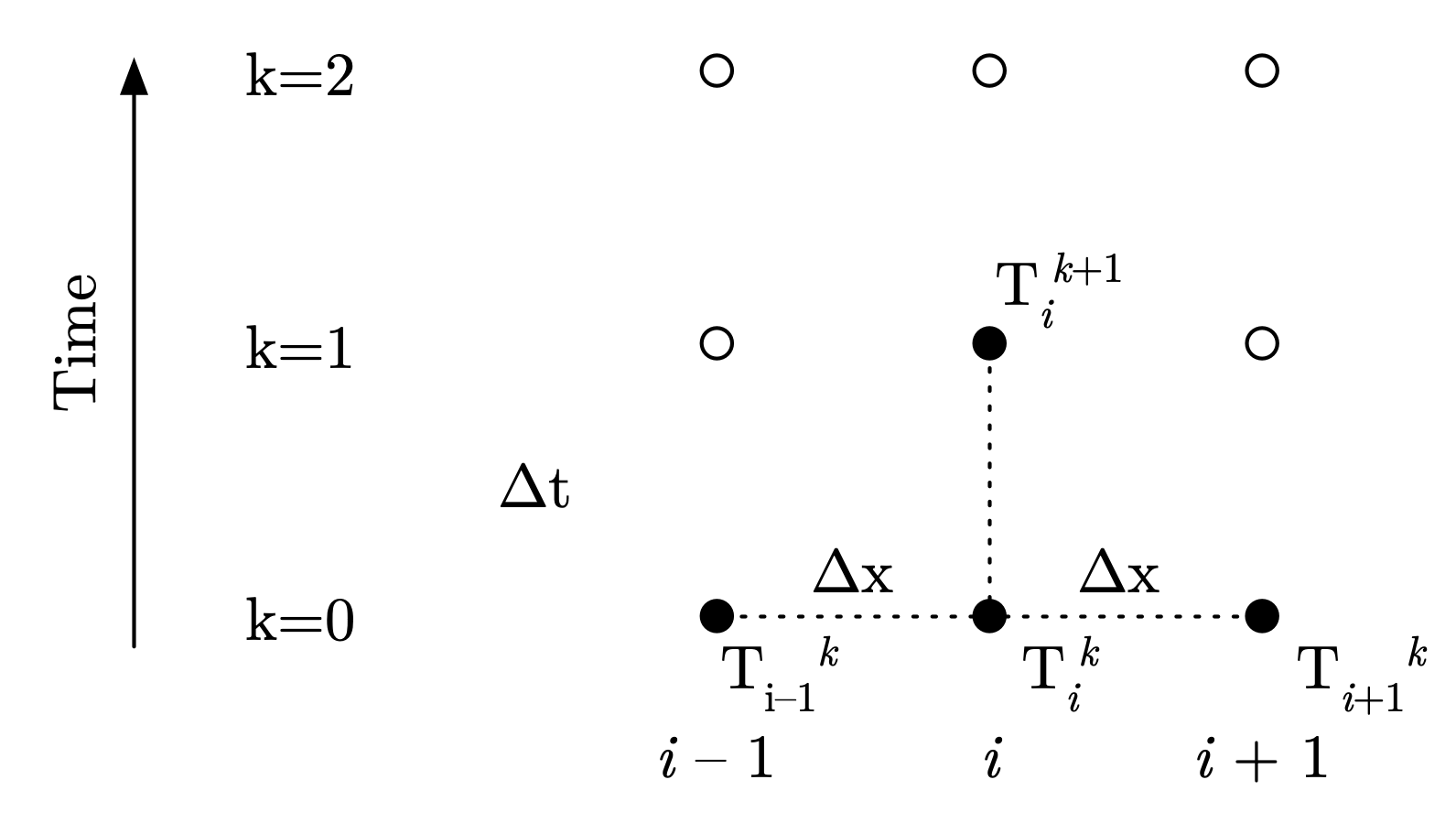
Fig. 5.7 Stencil for explicit solution to heat equation

To solve the heat equation for a one-dimensional domain over \(0 \leq x \leq L\), we will need both initial conditions at \(t = 0\) and boundary conditions at \(x=0\) and \(x=L\) (for all time). In terms of our nodal values, this means we need \(T_i^{k=0}\) for \(i = 0, \ldots, n-1\), where \(n\) is the number of points, as well as information about \(T_1^k\) and \(T_n^k\) for all times \(k\).

We can rearrange the above equation to obtain our recursion formula:

(5.28)\[\begin{equation} T_i^{k+1} = \left( T_{i+1}^k + T_{i-1}^k \right) \frac{\alpha \Delta t}{\Delta x^2} + T_i^k \left( 1 - 2 \frac{\alpha \Delta t}{\Delta x^2} \right) \;. \end{equation}\]

This is an explicit scheme in time, similar to the Forward Euler method we used for ordinary differential equations, and like that method it may have stability issues. The combination of terms we see repeated is also known as the Fourier number: \(\text{Fo} = \frac{\alpha \Delta t}{\Delta x^2}\), and governs the stability. We can rewrite the recursion formula using this:

(5.29)\[\begin{equation} T_i^{k+1} = \left( T_{i+1}^k + T_{i-1}^k \right) \text{Fo} + T_i^k \left( 1 - 2 \text{Fo} \right) \;. \end{equation}\]

The term in parentheses there must be greater than or equal to zero for stability (\(1 - 2 \text{Fo} \geq 0\)); if not, the solution may become unstable and blow up. This gives us some conditions on our choice of step sizes:

(5.30)\[\begin{align} 1 - 2 \text{Fo} &\geq 0 \\ 1 & \geq 2 \text{Fo} \\ \text{Fo} &\leq \frac{1}{2} \\ \frac{\alpha \Delta t}{\Delta x^2} &\leq \frac{1}{2} \end{align}\]

This is the stability criterion for the explicit method: the Fourier number must be smaller than 0.5. For a given thermal diffusivity and chosen spatial step size, this also gives us the limit on the time-step size: \(\Delta t \leq \Delta x^2 / (2 \alpha)\).

Let’s look at an example where the initial temperature is 200, the temperature at the boundaries are 50, the thermal diffusivity is \(\alpha = 2.3 \times 10^{-1}\) m\(^2 /\) s, and \(L = 1\). In other words,

(5.31)\[\begin{align} T(x, t=0) &= 200 \\ T(x=0, t) &= 50 \\ T(x=L, t) &= 50 \end{align}\]

We’ll integrate out to \(t = 1\), using a Fourier number of 0.25 to be comfortably below the stability limit (Fo = 0.25):

dx = 0.1
alpha = 2.3e-1

# for stability, set the Fourier number at 0.25 (half the limit of 0.5)
Fo_num = 0.25
# then choose time step size based on the Fourier number
dt = Fo_num * dx**2 / alpha

x_vals = np.arange(0, 1.001, dx)
times = np.arange(0, 1.0001, dt)

temps = np.zeros((len(times), len(x_vals)))

# initial conditions
temps[0,:] = 200

for k, t in enumerate(times[:-1]):
    for idx, x in enumerate(x_vals):
        if idx == 0 or idx == len(x_vals) - 1:
            # boundary conditions
            temps[k+1,idx] = 50
        else:
            temps[k+1,idx] = (
                (temps[k,idx+1] + temps[k,idx-1])*Fo_num +
                temps[k,idx] * (1 - 2*Fo_num)
                )

# create GIF of results

import matplotlib.animation as animation

fig, ax = plt.subplots()
ax.grid()
line, = ax.plot([], [], lw=2)
time_template = 'time = %.1f s'
time_text = ax.text(0.05, 0.9, '', transform=ax.transAxes)
ax.set_xlim([0, 1])
ax.set_ylim([50, 200])
ax.set_xlabel('distance')
ax.set_ylabel('temperature')

def animate(k):
    line.set_data((x_vals, temps[k,:]))
    time_text.set_text(time_template % (k*dt))
    return line, time_text

ani = animation.FuncAnimation(fig, animate, len(times), interval=20)

writer = animation.PillowWriter(fps=25)  
ani.save('parabolic_animated.gif', writer=writer)  

plt.close()

Fig. 5.8 Animated solution to 1D transient heat transfer PDE

This shows the temperature decaying exponentially from the initial conditions, constrained by the boundary conditions.

What happens if we tried to use a Fourier number larger than 0.5, or arbitrarily chose a time-step size that was too large (and resulted in \(\text{Fo} > 0.5\))?

dx = 0.1
alpha = 2.3e-1

# purposely choose a Fourier number past the stability limit
Fo_num = 0.75
dt = Fo_num * dx**2 / alpha

x_vals = np.arange(0, 1.001, dx)
times = np.arange(0, 1.0001, dt)

temps = np.zeros((len(times), len(x_vals)))

# initial conditions
temps[0,:] = 200

for k, t in enumerate(times[:-1]):
    for idx, x in enumerate(x_vals):
        if idx == 0 or idx == len(x_vals) - 1:
            # boundary conditions
            temps[k+1,idx] = 50
        else:
            temps[k+1,idx] = (
                (temps[k,idx+1] + temps[k,idx-1])*Fo_num +
                temps[k,idx] * (1 - 2*Fo_num)
                )

# create GIF of results

import matplotlib.animation as animation

fig, ax = plt.subplots()
ax.grid()
line, = ax.plot([], [], lw=2)
time_template = 'time = %.1f s'
time_text = ax.text(0.05, 0.9, '', transform=ax.transAxes)
ax.set_xlim([0, 1])
ax.set_ylim([50, 200])
ax.set_xlabel('distance')
ax.set_ylabel('temperature')

def animate(k):
    line.set_data((x_vals, temps[k,:]))
    time_text.set_text(time_template % (k*dt))
    return line, time_text

ani = animation.FuncAnimation(fig, animate, len(times), interval=20)

writer = animation.PillowWriter(fps=25)  
ani.save('parabolic_unstable_animated.gif', writer=writer)  

plt.close()

Fig. 5.9 Animated unstable solution

In this case, the solution becomes unstable and blows up, leading to unphysical results.

For this explicit scheme, the choice of \(\Delta t\) is limited by the stability criterion. This means that we may be stuck using a small time-step size.

Rather than being forced to use a very small time-step size, we can also explore implicit schemes that are unconditionally stable.

5.2.2. Implicit scheme

Recall that for solving initial value problems, when we ran into stability issues using explicit methods like forward Euler, we could use the backward Euler method to solve a problem with any time-step size. This worked by evaluating the derivative at the future/next step, and rearranging to get a recursion formula.

We can apply the same concept to parabolic PDEs like the unsteady heat equation, where the spatial derivatives are evaluated at the next time step:

(5.32)\[\begin{equation} \frac{T_{i-1}^{k+1} - 2 T_i^{k+1} + T_{i+1}^{k+1}}{\Delta x^2} = \frac{1}{\alpha} \left( \frac{T_i^{k+1} - T_i^k}{\Delta t} \right) \end{equation}\]

where, as before, \(T_i^k\) is the temperature at time \(t^k\) and spatial location \(x_i\). The following figure shows the stencil of points involved in the finite difference equation, applied to location \(x_i\) at time \(t^k\).

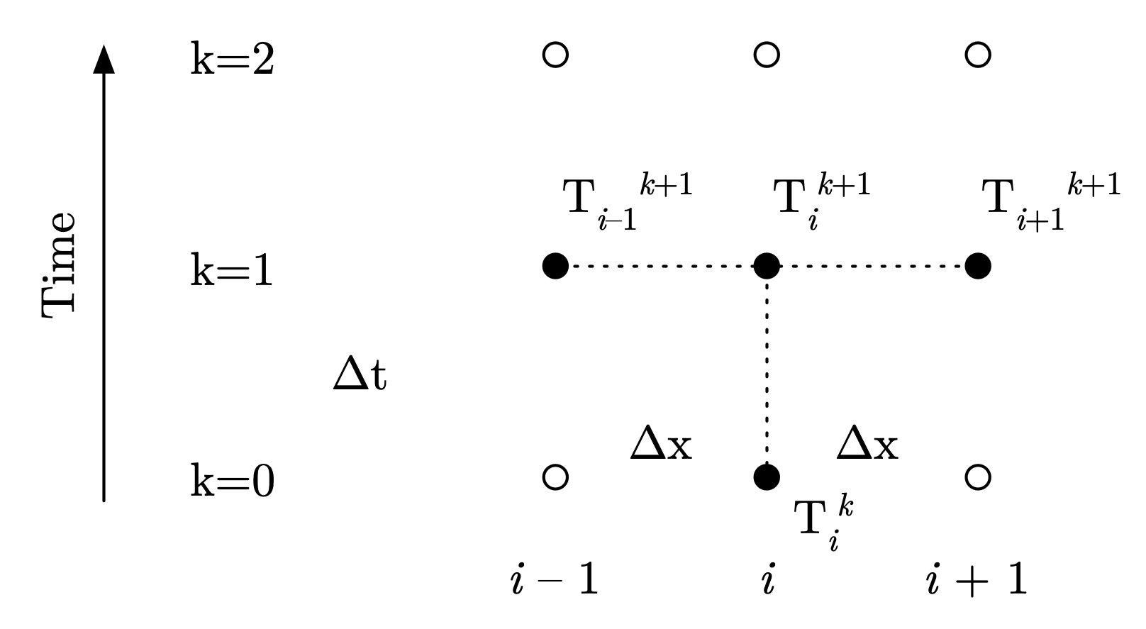
Fig. 5.10 Stencil for implicit solution to heat equation

Following the same process as with the explicit method, we can rearrange to get our recursion formula:

(5.33)\[\begin{equation} \left( -\text{Fo} \right) T_{i-1}^{k+1} + \left(1 + 2 \text{Fo} \right) T_i^{k+1} + \left( -\text{Fo} \right) T_{i+1}^{k+1} = T_i^k \;. \end{equation}\]

This is an implicit scheme in time, where the recursion formula involves more than one unknown. As a result, like with the backward Euler method, rather than simply calculating the new temperature at each location, we instead need to construct a system of equations to be solved simultaneously at each time step for all the locations:

(5.34)\[\begin{equation} A \mathbf{T}^{k+1} = \mathbf{T}^k = \mathbf{b} \;, \end{equation}\]

where \(\mathbf{T}^{k+1}\) is the array of unknowns. We can then solve using linear algebra, via the np.linalg.solve() function.

This method is unconditionally stable, meaning that the solution will not blow up for any combination of \(\Delta x\) and \(\Delta t\). Unfortunately, it’s a bit challenging to actually prove that with the tools we have, so we can instead demonstrate it:

# implicit scheme for solving the unsteady heat equation

dx = 0.1
alpha = 2.3e-1

# choose a Fourier number deliberately past the explicit method 
# stability limit to demonstrate unconditional stability
Fo_num = 0.75
# then choose time step size based on the Fourier number
dt = Fo_num * dx**2 / alpha

x_vals = np.arange(0, 1.001, dx)
times = np.arange(0, 1.0001, dt)

temps = np.zeros((len(times), len(x_vals)))

# initial conditions
temps[0,:] = 200

for k, t in enumerate(times[:-1]):
    A = np.zeros((len(x_vals), len(x_vals)))
    b = np.zeros(len(x_vals))
    for idx, x in enumerate(x_vals):
        if idx == 0 or idx == len(x_vals) - 1:
            # boundary conditions
            A[idx,idx] = 1
            b[idx] = 50
        else:
            A[idx,idx-1] = -Fo_num
            A[idx,idx] = 2*Fo_num + 1
            A[idx,idx+1] = -Fo_num
            b[idx] = temps[k,idx]
    temps[k+1,:] = np.linalg.solve(A, b)

# create GIF of results

import matplotlib.animation as animation

fig, ax = plt.subplots()
ax.grid()
line, = ax.plot([], [], lw=2)
time_template = 'time = %.1f s'
time_text = ax.text(0.05, 0.9, '', transform=ax.transAxes)
ax.set_xlim([0, 1])
ax.set_ylim([50, 200])
ax.set_xlabel('distance')
ax.set_ylabel('temperature')

def animate(k):
    line.set_data((x_vals, temps[k,:]))
    time_text.set_text(time_template % (k*dt))
    return line, time_text

ani = animation.FuncAnimation(fig, animate, len(times), interval=20)

writer = animation.PillowWriter(fps=25)  
ani.save('parabolic_implicit_animated.gif', writer=writer)  

plt.close()

Fig. 5.11 Solution to 1D heat equation with implicit method. Fo = 0.75

5.2.3. Crank-Nicolson scheme

So far we have two options for solving the unsteady heat equation (and parabolic PDEs in general): an explicit method and an implicit method. The explicit method is fairly easy to implement, but can suffer stability issues with larger time-step sizes. The implicit method offers unconditional stability, but at the cost of requiring linear algebra operations at each time step. Both schemes are first-order accurate in time, due to the first-order forward and backward differences used.

What do we do if we want a more-accurate solution, with less error?

The easiest thing is to reduce the time-step size. However, for realistic problems, typically we want to take the largest time-step size possible, to reduce how long the integration takes. This is particularly an issue with the implicit method, since the linear algebra operations can become quite expensive for larger problems.

Another option is to find a more-accurate method. The Crank-Nicolson method is second-order accurate in both space and time, and is also unconditionally stable.

This method works by averaging the spatial derivatives at both the current and next points in time:

(5.35)\[\begin{equation} \frac{1}{2} \left( \frac{T_{i-1}^k - 2 T_i^k + T_{i+1}^k}{\Delta x^2} \right) + \frac{1}{2} \left( \frac{T_{i-1}^{k+1} - 2 T_i^{k+1} + T_{i+1}^{k+1}}{\Delta x^2} \right) = \frac{1}{\alpha} \left( \frac{T_i^{k+1} - T_i^k}{\Delta t} \right) \end{equation}\]

The following figure shows the stencil of points involved in the finite difference equation, applied to location \(x_i\) at time \(t^k\), and involving six points:

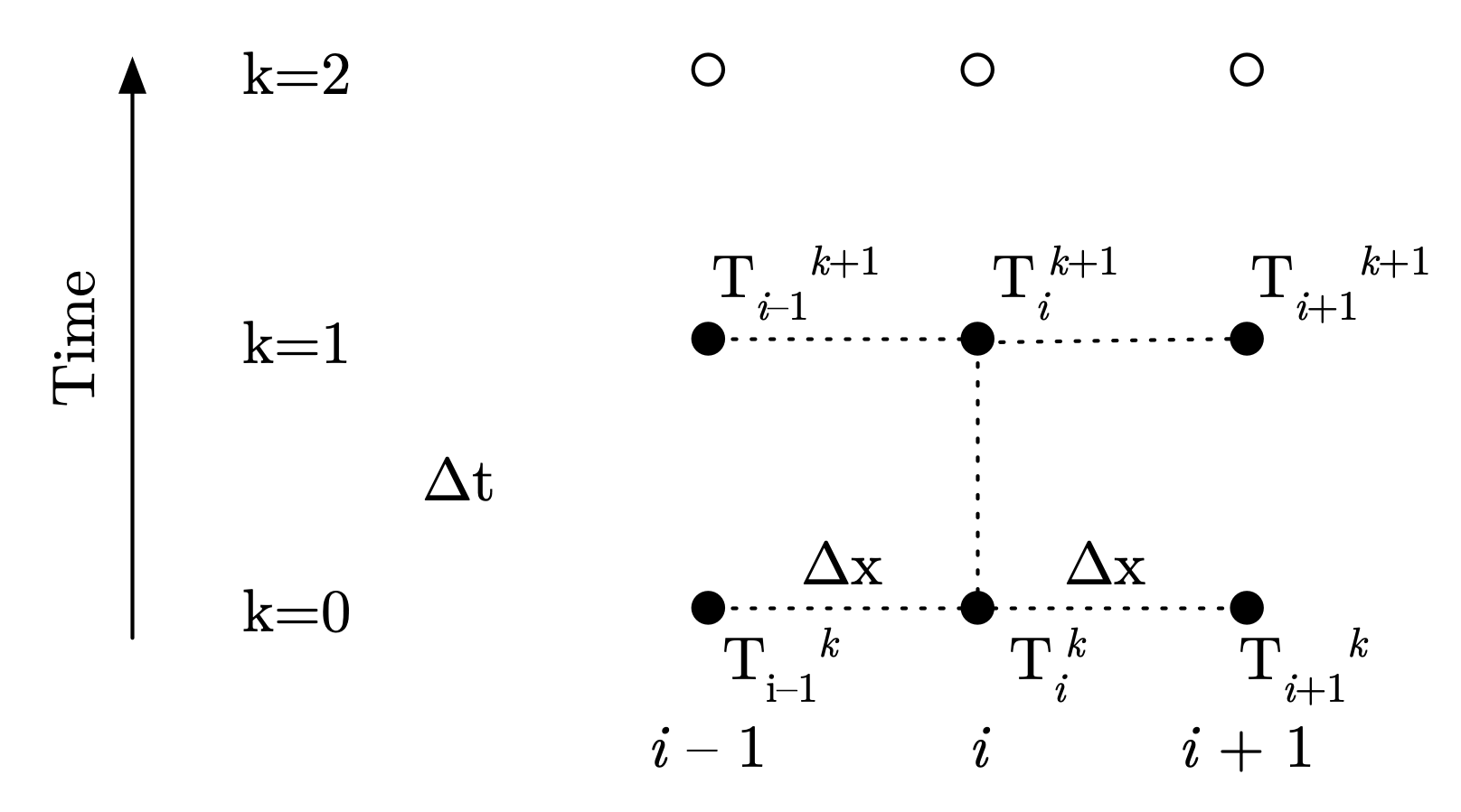
Fig. 5.12 Stencil for Crank–Nicolson solution to heat equation

We can rearrange to get our recursion formula:

(5.36)\[\begin{equation} -\text{Fo} \, T_{i-1}^{k+1} + \left(2 + 2 \text{Fo} \right) T_i^{k+1} - \text{Fo} \, T_{i+1}^{k+1} = \text{Fo} \, T_{i-1}^k + \left( -2 \text{Fo} + 2 \right) T_i^k + \text{Fo} \, T_{i+1}^k \;. \end{equation}\]

As with the first-order implicit scheme, each time step requires solving a simultaneous system of equations, which we can formulate as a linear algebra problem:

(5.37)\[\begin{equation} A \mathbf{T}^{k+1} = B \mathbf{T}^k = \mathbf{b} \;, \end{equation}\]

where \(\mathbf{T}^{k+1}\) is the array of unknowns. We can then solve using the np.linalg.solve() function.

# Crank-Nicolson scheme for solving the unsteady heat equation

dx = 0.1
alpha = 2.3e-1

# choose a Fourier number deliberately past the explicit method 
# stability limit to demonstrate unconditional stability
Fo_num = 0.75
# then choose time step size based on the Fourier number
dt = Fo_num * dx**2 / alpha

x_vals = np.arange(0, 1.001, dx)
times = np.arange(0, 1.0001, dt)

temps = np.zeros((len(times), len(x_vals)))

# initial conditions
temps[0,:] = 200

# set boundary conditions
temps[:,0] = 50
temps[:,-1] = 50

for k, t in enumerate(times[:-1]):
    A = np.zeros((len(x_vals), len(x_vals)))
    B = np.zeros((len(x_vals), len(x_vals)))
    for idx, x in enumerate(x_vals):
        if idx == 0 or idx == len(x_vals) - 1:
            # boundaries
            A[idx,idx] = 1
            B[idx,idx] = 1
        else:
            A[idx,idx-1] = -Fo_num
            A[idx,idx] = 2*Fo_num + 2
            A[idx,idx+1] = -Fo_num
            B[idx,idx-1] = Fo_num
            B[idx,idx] = -2*Fo_num + 2
            B[idx,idx+1] = Fo_num
    b = np.dot(B, temps[k, :])
    temps[k+1,:] = np.linalg.solve(A, b)

# create GIF of results

import matplotlib.animation as animation

fig, ax = plt.subplots()
ax.grid()
line, = ax.plot([], [], lw=2)
time_template = 'time = %.1f s'
time_text = ax.text(0.05, 0.9, '', transform=ax.transAxes)
ax.set_xlim([0, 1])
ax.set_ylim([50, 200])
ax.set_xlabel('distance')
ax.set_ylabel('temperature')

def animate(k):
    line.set_data((x_vals, temps[k,:]))
    time_text.set_text(time_template % (k*dt))
    return line, time_text

ani = animation.FuncAnimation(fig, animate, len(times), interval=20)

writer = animation.PillowWriter(fps=25)  
ani.save('parabolic_crank_nicolson_animated.gif', writer=writer)  

plt.close()

Fig. 5.13 Solution to 1D heat equation with Crank-Nicolson method. Fo = 0.75