Two-body problems¶

This module covers solution methods for two-body problems in the perifocal frame: given some information about an orbit, how can we find the new position and velocity after some change in true anomaly or after some time?

This will cover two-body problem solutions using Lagrange coefficients, Kepler problems (involving time), the Kepler problem with universal variables, and solving the orbital equation of motion numerically from initial conditions.

import numpy as np
%matplotlib inline
from matplotlib import pyplot as plt

# these lines are only for helping improve the display
from IPython.display import set_matplotlib_formats
set_matplotlib_formats('pdf', 'png')
plt.rcParams['figure.dpi']= 150
plt.rcParams['savefig.dpi'] = 150

Two-body problems in perifocal frame¶

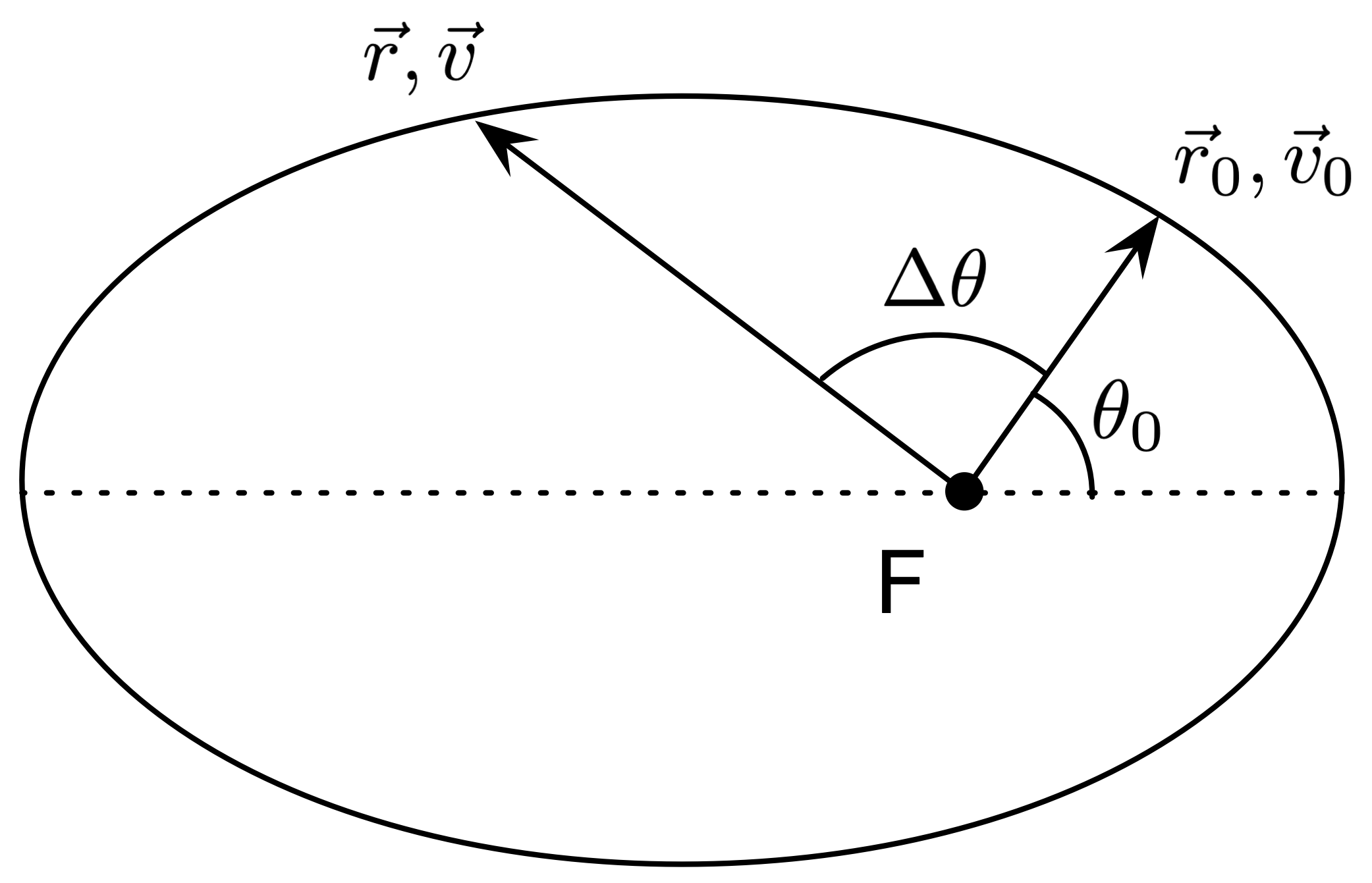
The problem: given the initial position vector \(\vec{r}_0\) and initial velocity vector \(\vec{v}_0\) (the state vectors), known at some instant in time, find the new state vectors \(\vec{r}\) and \(\vec{v}\) after the true anomaly changes by \(\Delta \theta\).

Fig. 3 Diagram of two-body problem with state vectors.¶

Since the state vectors \(\vec{r}\) and \(\vec{v}\) will always remain in the same two-dimensional plane, they must be able to be expressed as linear combinations of \(\vec{r}_0\) and \(\vec{v}_0\):

\[\begin{split} \begin{align} \vec{r} &= f \vec{r}_0 + g \vec{v}_0 \\ \vec{v} &= \dot{f} \vec{r}_0 + \dot{g} \vec{v}_0 \;, \end{align} \end{split}\]

where \(f, g, \dot{f}, \dot{g}\) are the Lagrange coefficients, which are constant scalars.

Note that by substituting these into the definition of specific angular momentum \(\vec{h}\), which must remain constant, we can obtain the Lagrange identity:

\[\begin{split} \begin{align} \vec{h} = \vec{r}_0 \times \vec{v}_0 &= \vec{r} \times \vec{v} \\ &= \left( f \vec{r}_0 + g \vec{v}_0 \right) \times \left( \dot{f} \vec{r}_0 + \dot{g} \vec{v}_0 \right) \\ &= f \dot{f} \vec{r}_0 \times \vec{r}_0 + f \dot{g} \vec{r}_0 \times \vec{v}_0 + g \dot{f} \vec{v}_0 \times \vec{r}_0 + g \dot{g} \vec{v}_0 \times \vec{v}_0 \\ &= f \dot{g} \vec{r}_0 \times \vec{v}_0 + g \dot{f} \vec{v}_0 \times \vec{r}_0 \\ &= f \dot{g} \vec{r}_0 \times \vec{v}_0 - g \dot{f} \vec{r}_0 \times \vec{v}_0 \\ \vec{r}_0 \times \vec{v}_0 &= \left( f \dot{g} - g \dot{f} \right) \vec{r}_0 \times \vec{v}_0 \\ \therefore f \dot{g} - g \dot{f} &= 1 \;, \end{align} \end{split}\]

which provides a potentially helpful relationship between the coefficients—given three of them, you can easily find the fourth.

Lagrange coefficients¶

Via a complicated derivation, we can find closed-form expressions for the Lagrange coefficients:

(3)¶\[\begin{split} \begin{align} f &= 1 - \frac{\mu r}{h^2} \left( 1 - \cos \Delta \theta \right) \\ g &= \frac{r r_0}{h} \sin \Delta \theta \\ \dot{f} &= \frac{\mu}{h} \frac{1 - \cos \Delta \theta}{\sin \Delta \theta} \left[ \frac{\mu}{h^2} \left( 1 - \cos \Delta \theta \right) - \frac{1}{r_0} - \frac{1}{r} \right] \\ \dot{g} &= 1 - \frac{\mu r_0}{h^2} \left( 1 - \cos \Delta \theta \right) \;, \end{align} \end{split}\]

where \(r_0 = |\vec{r}_0| = \sqrt{\vec{r}_0 \cdot \vec{r}_0}\) is the magnitude of the initial position vector, \(v_0 = |\vec{v}_0| = \sqrt{\vec{v}_0 \cdot \vec{v}_0}\) is the magnitude of the initial velocity vector, \(v_{r0} = \vec{r}_0 \cdot \vec{v}_0 / r_0\) is the radial component of the initial velocity vector (the projection along the apse line), \(h = |\vec{h}|\) is the magnitude of the specific angular momentum, and the new radial distance is

\[ r = \frac{h^2}{\mu} \frac{1}{1 + \left( \frac{h^2}{\mu r_0} - 1 \right) \cos \Delta \theta - \frac{h v_{r0}}{\mu} \sin \Delta \theta} \;. \]

Note

While examples may show elliptical orbits, this approach applies regardless of orbit.

With these equations, we can now solve the problem.

Example workflow¶

The workflow for solving a problem follows these steps:

Calculate the magnitudes and necessary quantities: \(r_0 = |\vec{r}_0|\), \(v_0 = |\vec{v}_0|\), \(\vec{h} = \vec{r} \times \vec{v}\), \(h = |\vec{h}|\), and \(v_{r0} = \frac{ \vec{r}_0 \cdot \vec{v}_0 }{ |r_0| }\).
An optional step is to determine the initial true anomaly, and from that the eccentricity of the orbit \(e\) (which would tell us what kind of orbit this is):

\[\begin{split} \begin{align} \theta_0 &= \tan^{-1} \left( \frac{r_{0y}}{r_{0x}} \right) \\ r_0 &= \frac{h^2 / \mu}{1 + e \cos \theta_0 } \\ \rightarrow e &= \left( \frac{h^2 / \mu}{r_0} - 1 \right) / \cos \theta_0 \end{align} \end{split}\]
Calculate the new radial distance:

\[ r = \frac{h^2}{\mu} \frac{1}{1 + \left( \frac{h^2}{\mu r_0} - 1 \right) \cos \Delta \theta - \frac{h v_{r0}}{\mu} \sin \Delta \theta } \]
Calculate the Lagrange coefficients \(f, g, \dot{f}, \dot{g}\), using Equation (3).
Finally, calculate the new position and velocity vectors:

\[\begin{split} \begin{align} \vec{r} &= f \vec{r}_0 + g \vec{v}_0 \\ \vec{v} &= \dot{f} \vec{r}_0 + \dot{g} \vec{v}_0 \end{align} \end{split}\]

Here’s example code in Matlab and Python for doing these steps:

matlab

mu = 398.6e3; % km^3/s^2
r0 = [. . .];
v0 = [. . .];
delta_theta = .;

% 1. Calculate magnitudes
r0_mag = sqrt(dot(r0, r0));
v0_mag = sqrt(dot(v0, v0));

h = cross(r0, v0);
h_mag = sqrt(dot(h, h));
v_r0 = dot(r0, v0) / r0_mag;

% 2. Get eccentricity
theta_0 = atan(r0(2) / r0(1));
e = ((h_mag^2/(mu * r0_mag)) - 1) / cos(theta_0);

% 3. Get new distance
r_mag = (h_mag^2/mu) / (1 + ((h_mag^2/(mu*r0_mag)) - 1)*cos(delta_theta) - h_mag*v_r0 * sin(delta_theta)/mu);

% 4. Get Lagrange coefficients
f = 1 - mu * r_mag * (1 - cos(delta_theta)) / h_mag^2;
g = r_mag * r0_mag * sin(delta_theta) / h_mag;
fdot = (mu / h_mag)*(1 - cos(delta_theta))*( mu*(1 - cos(delta_theta))/h_mag^2 - (1/r0_mag) - (1/r_mag)) / sin(delta_theta);
gdot = 1 - mu*r0_mag*(1 - cos(delta_theta)) / h_mag^2;

% 5. Calculate new vectors:
r = f*r0 + g*v0;
v = fdot*r0 + gdot*v0;

python

import numpy as np

mu = 398.6e3 # km^3/s^2
r0 = np.array([. . .])
v0 = np.array([. . .])
delta_theta = .

# 1. Calculate magnitudes
r0_mag = np.sqrt(np.dot(r0, r0))
v0_mag = np.sqrt(np.dot(v0, v0))

h = np.cross(r0, v0)
h_mag = np.sqrt(np.dot(h, h))
v_r0 = np.dot(r0, v0) / r0_mag

# 2. Get eccentricity
theta_0 = np.arctan(r0[1] / r0[0])
e = ((h_mag^2/(mu * r0_mag)) - 1) / np.cos(theta_0)

# 3. Get new distance
r_mag = (h_mag^2/mu) / (
    1 + ((h_mag^2/(mu*r0_mag)) - 1)*np.cos(delta_theta) - h_mag*v_r0 * np.sin(delta_theta)/mu
    )

# 4. Get Lagrange coefficients
f = 1 - mu * r_mag * (1 - np.cos(delta_theta)) / h_mag^2
g = r_mag * r0_mag * np.sin(delta_theta) / h_mag
fdot = (mu / h_mag)*(1 - np.cos(delta_theta))*(
    mu*(1 - np.cos(delta_theta))/h_mag^2 - (1/r0_mag) - (1/r_mag)
    ) / np.sin(delta_theta)
gdot = 1 - mu*r0_mag*(1 - np.cos(delta_theta)) / h_mag^2

# 5. Calculate new vectors:
r = f*r0 + g*v0
v = fdot*r0 + gdot*v0

Kepler problems¶

Kepler problems are two-body problems that involve time: find the time of flight given information about an orbit and a change in true anomaly, or find the change in true anomaly (and new state vectors) given a time of flight.

Example: find time of flight¶

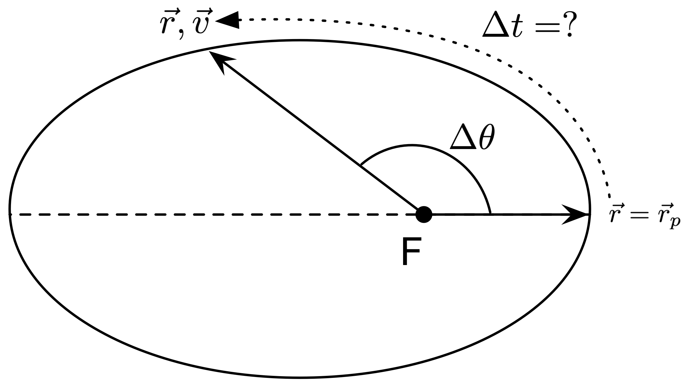
The problem: Given the orbital eccentricity \(e\), the initial position vector \(\vec{r} = \vec{r}_p\) (the position starts at perigee), and the change in true anomaly \(\Delta \theta\), find the time of flight \(\Delta t\). (The solution procedure does not depend on the initial position being at perigee, this is just to simplify things a bit.)

Fig. 4 Diagram of Kepler problem for finding time of flight.¶

This problem requires a different approach. We can relate the transverse/angular component of velocity to the change in true anomaly:

(4)¶\[\begin{split} \begin{align} V_{\theta} = \frac{h}{r} &= r \dot{\theta} = r \frac{d\theta}{dt} \\ r^2 \, d\theta &= h \, dt \\ \text{but } r &= \frac{h^2 / \mu}{1 + e \cos \theta} \\ \rightarrow \left( \frac{h^2 / \mu}{1 + e \cos \theta} \right)^2 d\theta &= h \, dt \\ \int_{\theta_0 = 0}^{\theta = \Delta \theta} \left( \frac{1}{1 + e \cos \theta} \right)^2 d\theta &= \int_0^t \frac{\mu^2}{h^3} dt \\ \end{align} \end{split}\]

This is the Kepler integral, and it has a closed-form solution! (Fortunately, the bounds of the integral do not matter—just the \(\Delta \theta\).)

However, depending on the value of eccentricity \(e\), the solution takes on different forms. So this approach depends on knowing eccentricity! We will cover a more-general method that does not require this information soon.

For an elliptic orbit, the solution to the Kepler integral is

\[\begin{split} \begin{align} \frac{2 \pi}{T} t &= M_e = E - e \sin E \\ \tan \frac{E}{2} &= \sqrt{\frac{1-e}{1+e}} \tan \frac{\Delta \theta}{2} \;, \end{align} \end{split}\]

where \(T\) is the period of an elliptical orbit, \(E\) is the eccentric anomaly (which must be in radians), and \(M_e\) is the mean anomaly.

Warning

Make sure you use the correct form of the equations based on the value of eccentricity! And make sure your anomaly values are in radians!

The solution procedure for solving this problem is then:

Calculate the magnitude of specific angular momentum \(h\) using the known perigee distance:

\[ r_p = \frac{h^2 / \mu}{1 + e} \rightarrow h \]
Calculate the apogee distance, and then use this to get the semi-major axis:

\[\begin{split} \begin{align} r_a &= \frac{h^2 / \mu}{1 - e} \\ a &= \frac{r_p + r_a}{2} \end{align} \end{split}\]
For an elliptic orbit, calculate the period:

\[ T = \frac{2\pi}{\sqrt{\mu}} a^{3/2} \]
Calculate the eccentric anomaly \(E\), and then use this to get \(t\).

Example: find change in true anomaly¶

The problem: now, given the eccentricity \(e\), initial position vector \(\vec{r}=\vec{r}_p\), and the time of flight \(\Delta t\), find the associated change in true anomaly \(\Delta \theta\), and then the new state vectors (\(\vec{r}\) and \(\vec{v}\)).

As we will quickly see, this problem is a bit trickier, but still solveable.

The following solution steps for an elliptic orbit, since the equations only apply for this case, but the procedure will be the same for other orbits:

Calculate the semi-major axis \(a\) and orbital period \(T\) using the perigee distance.
Calculate the mean anomaly using the known time of flight:

\[ M_e = \frac{2\pi}{T} t \]

Next, we need to to find the eccentric anomaly \(E\), using the \(M_e = E - e \sin E\), but this is a transcendental equation with no closed-form solution. So, we need to use an iterative solution procedure, for example using the fzero() function in Matlab or the scipy.optimize.root_scalar() function in Python (which requires SciPy). Either way, we need a good initial guess, otherwise even these robust algorithms may not converge to the correct solution.

Use the Prussing estimate as a reasonable first guess for \(E\):

\[ E_0 = M_e + \frac{e}{2} \;. \]

Then, use an equation solver to find \(E\):

matlab

E0 = M_e + e/2;
E = fzero(@f, E0);

function zero = f(E)
  M_e = 2 * pi * t / T;
  zero = M_e - (E - e * sin(E));
end

python

import numpy as np
from scipy.optimize import root_scalar

def eccentric_anomaly(E):
    M_e = 2 * np.pi * t / T
    return M_e - (E - e * np.sin(E))

E0 = M_e + e/2
sol = root_scalar(eccentric_anomaly, x0=E0)

Use \(E\) to find the value of the change in true anomaly:

\[ \tan \frac{\Delta \theta}{2} = \sqrt{\frac{1+e}{1-e}} \tan \frac{E}{2} \;. \]
Then, with \(\Delta \theta\), you can find the new state vectors by treating this like a two-body problem and using the Lagrange coefficients. Since this example starts at perigee, we know the initial position and velocity vectors:

\[\begin{split} \begin{align} \vec{r}_0 &= \vec{r}_p = \left[ r_p, 0, 0 \right] \\ \vec{v}_0 &= \left[ 0, \frac{h}{r_p}, 0 \right] \end{align} \end{split}\]

Universal variable approach¶

The above approaches are all limited by the need to know the eccentricity of the orbit, which in general you would not know. The universal variable approach is a more-general approach that applies consistently regardless of orbital eccentricity.

The problem: Given initial position vector \(\vec{r}_0\), initial velocity vector \(\vec{v}_0\), and some time of flight \(\Delta t\), find the new state vectors \(\vec{r}\) and \(\vec{v}\).

This approach is based on the definition of the universal anomaly \(\chi\), using:

\[ \dot{\chi} \equiv \frac{\sqrt{\mu}}{r} \;, \]

known as the Sundmann transformation.

Through a complicated derivation, this leads to the universal variable formulation of Kepler’s equation:

\[ \sqrt{\mu} \Delta t = \frac{r_0 v_{r0}}{\sqrt{\mu}} \chi^2 C \left( \alpha \chi^2 \right) + (1 - \alpha r_0) \chi^3 S \left( \alpha \chi^2 \right) + r_0 \chi \;, \]

which is a highly nonlinear transcendental equation, where \(\alpha = \frac{1}{a} = \frac{2}{r_0} - \frac{v_0^2}{\mu}\). But, this is solveable via iterative methods!

However, as above, we need a good first guess to help the solvers converge, and we also need to define the functions \(C()\) and \(S()\).

First, we can get a first guess for \(\chi\) using the Chobotov approximation:

\[ \chi_0 = \frac{\sqrt{\mu}}{|a|} \Delta t \;. \]
Then, we need to define the Stumpff functions:

\[\begin{split} \begin{align} C(z) &= \frac{\cosh \left(\sqrt{-z}\right) - 1}{-z} \\ S(z) &= \left\lvert \frac{ \sinh \left(\sqrt{-z}\right) - \sqrt{-z}}{ \left(\sqrt{-z}\right)^3 } \right\rvert \;, \end{align} \end{split}\]

where \(z = \alpha \chi^2\). Take care to include the absolute value when evaluating \(S(z)\), which must be positive.
Then, solve iteratively for \(\chi\), using (for example) fzero() in Matlab or scipy.optimize.root_scalar() in Python.
Once you obtain \(\chi\), you can solve for the Lagrange coefficients \(f\) and \(g\) with the universal Lagrange equations:

\[\begin{split} \begin{align} f &= 1 - \frac{\chi^2}{r_0} C \left( \alpha \chi^2 \right) \\ g &= \Delta t - \frac{1}{\sqrt{\mu}} \chi^3 S \left( \alpha \chi^2 \right) \;. \end{align} \end{split}\]

Then, calculate the new position vector: \(\vec{r} = f \vec{r}_0 + g \vec{v}_0\).
Calculate the magnitude of \(\vec{r}\): \(|\vec{r}|\).
Then, we can get \(\dot{f}\) and \(\dot{g}\) to find the velocity vector:

\[\begin{split} \begin{align} \dot{f} &= \frac{\sqrt{\mu}}{r r_0} \left[ \alpha \chi^3 S \left( \alpha \chi^2 \right) - \chi \right] \\ \dot{g} &= 1 - \frac{\chi^2}{r} C \left( \alpha \chi^2 \right) \\ \vec{v} &= \dot{f} \vec{r}_0 + \dot{g} \vec{v}_0 \;. \end{align} \end{split}\]

Solve equation of motion numerically¶

An alternate strategy for finding the position and velocity of an orbiting body after some time of flight, given the initial position and velocity, is to numerically integrate the orbital equation of motion:

\[ \vec{ \ddot{r} } + \frac{\mu}{r^3} \vec{r} = 0 \;, \]

based on initial conditions \(\vec{r}_0\) and \(\vec{v}_0\) defined at an initial time \(t_0\). Integrating this forward in time would give us the position as a function of time: \(x(t)\), \(y(t)\), and \(z(t)\).

If you recall the methods for integrating second-order ordinary differential equations (ODEs), we can solve this by decomposing it into six first-order ODEs:

\[\begin{split} \begin{align} z_1 &= x \rightarrow \dot{z}_1 = z_4 \\ z_2 &= y \rightarrow \dot{z}_2 = z_5 \\ z_3 &= z \rightarrow \dot{z}_3 = z_6 \\ z_4 &= \dot{x} \rightarrow \dot{z}_4 = \ddot{x} = -\frac{\mu}{r^3} z_1 \\ z_5 &= \dot{y} \rightarrow \dot{z}_5 = \ddot{y} = -\frac{\mu}{r^3} z_2 \\ z_6 &= \dot{z} \rightarrow \dot{z}_6 = \ddot{z} = -\frac{\mu}{r^3} z_3 \;, \end{align} \end{split}\]

where the radial position magnitude is \(r = \sqrt{z_1^2 + z_2^2 + z_3^2}\).

We can then integrate using ode45() in Matlab, or solve_ivp() in Python/SciPy:

matlab

clear, clf, clc;

r0 = [. . .];
v0 = [. . .];
T = .;

options = odeset('RelTol', 1e-6);

[T, Z] = ode45(@rhs, [0 2*T], [r0, v0], options);
plot3(Z(:,1), Z(:,2), Z(:,3));

% function for ODE system
function dzdt = rhs(t, z)
  mu = 398.6e3; % km^3/s^2
  r = sqrt(z(1)^2 + z(2)^2 + z(3)^2);
  dzdt = zeros(6,1);
  dzdt(1) = z(4);
  dzdt(2) = z(5);
  dzdt(3) = z(6);
  dzdt(4) = (-mu/r^3) * z(1);
  dzdt(5) = (-mu/r^3) * z(2);
  dzdt(6) = (-mu/r^3) * z(3);
end

python

import numpy as np
from scipy.integrate import solve_ivp
import matplotlib.pyplot as plt

def rhs(t, z):
    # 3D orbital motion ODE
    mu = 398.6e3 # km^3/s^2
    r = np.sqrt(z[0]**2 + z[1]**2 + z[2]**2)
    dzdt = np.zeros(6)
    dzdt[0] = z[3]
    dzdt[1] = z[4]
    dzdt[2] = z[5]
    dzdt[3] = (-mu/r**3) * z[0]
    dzdt[4] = (-mu/r**3) * z[1]
    dzdt[5] = (-mu/r**3) * z[2]
    return dzdt
    
r0 = [. . .]
v0 = [. . .]
T = .

sol = solve_ivp(rhs, [0, 2*T], np.array(r0 + v0))

fig = plt.figure()
ax = fig.add_subplot(111, projection='3d')
ax.plot3D(sol.y[0,:], sol.y[1,:], sol.y[2.:])

Summary of Kepler’s equations¶

Fig. 5 Diagram showing the geometric meaning of the mean and eccentric anomaly. Original sources: PNG by Brews ohare, SVG by CheCheDaWaff. Shared under CC BY-SA¶

Elliptic orbit¶

\[\begin{split} \begin{align} M_e &= \frac{2 \pi}{T} t = \sqrt{\frac{\mu}{a^3}} t \\ M_e &= E - e \sin E \\ \tan \frac{\theta}{2} &= \sqrt{\frac{1+e}{1-e}} \tan \frac{E}{2} \\ r &= a \left( 1 - e \cos E \right) \\ v^2 &= \mu \left( \frac{2}{r} - \frac{1}{a} \right) \\ r_p &= a (1 - e) \;, \end{align} \end{split}\]

where \(M_e\) is the mean anomaly and \(E\) is the eccentric anomaly.

Hyperbolic orbit¶

\[\begin{split} \begin{align} M_h &= \sqrt{\frac{\mu}{(-a)^3}} \, t = \frac{\mu^2}{h^3} \left( e^2 - 1 \right)^{3/2} t\\ M_h &= e \sinh F - F \\ \tan \frac{\theta}{2} &= \sqrt{\frac{e+1}{e-1}} \tanh \frac{F}{2} \\ r &= a \left( 1 - e \cosh F \right) \\ v^2 &= \mu \left( \frac{2}{r} - \frac{1}{a} \right) \\ r_p &= a (1 - e) \;, \end{align} \end{split}\]

where \(M_h\) is the mean anomaly and \(F\) is the hyperbolic anomaly.

Space Systems Engineering notes

Two-body problems¶

Two-body problems in perifocal frame¶

Lagrange coefficients¶

Example workflow¶

Kepler problems¶

Example: find time of flight¶

Example: find change in true anomaly¶

Universal variable approach¶

Solve equation of motion numerically¶

Summary of Kepler’s equations¶

Elliptic orbit¶

Hyperbolic orbit¶