Introduction to orbital mechanics: conic sections¶

Orbital mechanics refers to the study of motion due to the gravitational influence of one mass over another. To start, we’ll focus on unperturbed orbits mostly of satellites around Earth, meaning orbits that result only from the force of gravity from a larger body, and without the influence of

thrust forces
gravitational perturbations
irregularities in the Earth’s radius

To determine what orbits are possible, we need to derive the orbital equation of motion.

import numpy as np
%matplotlib inline
from matplotlib import pyplot as plt

# these lines are only for helping improve the display
from IPython.display import set_matplotlib_formats
set_matplotlib_formats('pdf', 'png')
plt.rcParams['figure.dpi']= 150
plt.rcParams['savefig.dpi'] = 150

Orbital equation of motion¶

For now, we will focus on orbital problems involving two bodies (i.e., the two-body problem), with two different masses, usually where one is much larger than the other, such as a satellite orbiting the Earth.

We will also focus on orbital motion in the two-dimensional perifocal frame, where all motion remains in the same two-dimensional plane with the two masses.

$\vec{R_1}$ and $\vec{R_2}$ are the position vectors for masses $M_1$ and $M_2$, respectively, from some absolute frame of reference, and then we can define the relative position vector from $M_1$ to $M_2$ as $\vec{r} = \vec{R_2} - \vec{R_1}$.

These masses act on each other via the force of gravity—this is reciprocal, in that each mass acts on the other. Newton’s gravitational law states that this force is

(1)¶\[ F_{12} = G \frac{m_1 m_2}{r^2} = -F_{21} \;, \]

where $r^2 = | \vec{r} |$ and $G = 6.674 \cdot 10^{-11}$ m³/(kg s²), the universal gravitational constant.

If we take the time derivative of $\vec{r}$ twice, we get the acceleration vector, and can substitute $\vec{F} = m \vec{a}$ with Equation (1):

\[\begin{split} \begin{align} \vec{\ddot{r}} &= \vec{\ddot{R}}_2 - \vec{\ddot{R}}_1 \\ \vec{\ddot{r}} &= -G \left( \frac{m_1 m_2}{r^2} \right) \left( \frac{1}{m_1} + \frac{1}{m_2} \right) \vec{u}_r \;, \end{align} \end{split}\]

where $\vec{u}_r = \frac{\vec{r}}{|\vec{r}|}$ is the unit direction vector. Since the masses involved, and gravitational constant, do not change for a given orbital system, we can simplify this by defining the gravitational parameter $\mu$:

\[ G (m_1 + m_2) \approx G m_1 \equiv \mu \;, \]

where $m_1$ is the mass of the central body (e.g, Earth) and $m_2$ is the mass of the orbiting body, and $m_2 \ll m_1$. For a given planetary orbit, this parameter does not change, and for an Earth-satellite system $\mu = 398,600 \, \text{km}^3/\text{s}^2$.

Then, we can express the orbital equation of motion as

(2)¶\[ \vec{\ddot{r}} = -\frac{\mu}{r^3} \vec{r} \;, \]

where $r = |\vec{r}| = \sqrt{r_x^2 + r_y^2 + r_z^2}$ is the magnitude of the radial distance. This is a vector, nonlinear, second-order ordinary differential equation. We can solve this numerically by decomposing into a system of six first-order equations, but we can also study orbits in a two-dimensional plane.

The goal of any solution approach is to obtain the state vectors of position and velocity, $\vec{r}(t)$ and $\vec{v}(t)$, which are both functions of time.

Specific angular momentum¶

Now that we know the equation governing orbital motion, and understand that this comes from Newton’s law of gravitation, we can see that in a general orbit, many quantities will constantly be changing: position, velocity, and force. While these things are constantly changing, we will see that specific angular momentum remains constant:

\[ \vec{h} = \vec{r} \times \vec{v} \;, \]

which is likely the single-most important quantity in orbital mechanics/astrodynamics. Note $\vec{r}$ and $\vec{v}$ form an orbital plane, and $\vec{h}$ is perpendicular to this plane.

We can show that specific angular momentum remains constant by taking the cross product of the orbital equation of motion with the position vector:

\[\begin{split} \begin{align} \vec{r} \times \vec{\ddot{r}} + \vec{r} \times \frac{\mu}{r^3} \vec{r} &= 0 \quad \text{but } \vec{r} \times \vec{r} = 0 \\ \rightarrow \vec{r} \times \vec{\ddot{r}} &= 0 \;. \\ \text{Then, } \frac{d\vec{h}}{dt} = \frac{d}{dt} \left( \vec{r} \times \vec{v} \right) &= \frac{d}{dt} \left( \vec{r} \times \vec{\dot{r}} \right) \\ \text{Product rule: } \frac{d\vec{h}}{dt} = \vec{\dot{r}} \times \vec{\dot{r}} + \vec{r} \times \vec{\ddot{r}} &= \vec{r} \times \vec{\ddot{r}} \\ \therefore \frac{d\vec{h}}{dt} = \vec{r} \times \vec{\ddot{r}} &= 0 \;. \end{align} \end{split}\]

Therefore, $\vec{h}$ is constant, while position, velocity, and force/acceleration may change.

Orbit equation¶

If we know the specific angular momentum, it would be helpful to relate this to position and velocity for a specific orbit. We can obtain a useful relation by taking the cross product of the orbital equation of motion with angular momentum:

\[\begin{split} \begin{align} \vec{\ddot{r}} \times \vec{h} + \frac{\mu}{r^3} \left(\vec{r} \times \vec{h}\right) &= 0 \\ \text{but } \frac{d}{dt} \left( \vec{\dot{r}} \times \vec{h} \right) &= \vec{\ddot{r}} \times \vec{h} + \vec{\dot{r}} \times \vec{\dot{h}} = \vec{\ddot{r}} \times \vec{h} \\ \rightarrow \frac{d}{dt} \left( \vec{\dot{r}} \times \vec{h} \right) + \frac{\mu}{r^3} \left[ \vec{r} \times \left( \vec{r} \times \vec{v} \right) \right] &= 0 \\ \text{via law of triple cross products: } \frac{d}{dt} \left( \vec{\dot{r}} \times \vec{h} \right) &= \frac{\mu}{r^3} \left[ \vec{\dot{r}} r^2 - \vec{r} \left(\vec{r} \cdot \vec{\dot{r}} \right) \right] \\ \int \frac{d}{dt} \left( \vec{\dot{r}} \times \vec{h} \right) &= \mu \int \frac{d}{dt} \left( \frac{\vec{r}}{|r|} \right) \\ \vec{\dot{r}} \times \vec{h} &= \frac{\mu}{r} \vec{r} + \vec{C} \;, \end{align} \end{split}\]

where $\vec{C}$ is a vector constant of integration. We can obtain a scalar equation by taking the dot product of the last result with the position vector:

\[\begin{split} \begin{align} \vec{r} \cdot \left( \vec{\dot{r}} \times \vec{h} \right) &= \mu \left( \vec{r} \cdot \frac{\vec{r}}{|r|} \right) + \vec{r} \cdot \vec{C} \\ \text{but } \vec{r} \cdot \vec{\dot{r}} \times \vec{h} = \vec{r} \cdot \vec{v} \times \vec{h} &= \vec{r} \times \vec{v} \cdot \vec{h} = \vec{h}\cdot\vec{h} = h^2 \\ \rightarrow h^2 &= \mu r + r \, C \cos \theta \\ \frac{h^2}{\mu} &= r \left( 1 + \frac{C}{\mu} \cos \theta \right) \\ \therefore r &= \frac{h^2 / \mu}{1 + e \cos \theta} \;, \end{align} \end{split}\]

where $\theta$ is the angle between $\vec{r}$ and $\vec{C}$, called the true anomaly (and also referred to with the variable $\nu$ in some places), and $e = \frac{C}{\mu}$ is the eccentricity. The is the orbit equation, and it tells us the radial distance for a given location in orbit, based on a magnitude of angular momentum.

Now that we have an equation for the shape of any orbit, we can look at the different kinds of orbits that are possible. The orbital equation above describes a family of curves called conic sections, because they can be formed by taking two-dimensional slices of three-dimensional opposed cones:

Fig. 1 Depiction of the conic sections: circle, ellipse, parabola, and hyperbola. Source: Kelvinsong / CC BY-SA, hosted on Wikimedia Commons.¶

We can see that four orbital shapes are possible, depending on the value of eccentricity $e$:

$e = 0$: circular orbit, which is a special case of an ellipse. GPS satellites have nearly circular orbits ($e < 0.02$), to keep nearly a constant radial distance from the surface.
$0 < e < 1$: elliptical orbit. This is the shape of planetary orbits, and nearly all stable orbits are elliptical.
$e = 1$: parabolic orbit. This is unnatural, and we generally won’t discuss this type of orbit.
$e > 1$: hyperbolic orbit. This is a so-called flyby orbit, where the satellite/orbiting object comes in close and then leaves.

Velocity components¶

Fig. 2 Position and velocity vectors of an object orbiting a central body, showing the flight-path angle $\nu = \theta$. Source: Åntøinæ / CC BY-SA, hosted on Wikimedia Commons.¶

The velocity vector can be broken into two components, in the radial and angular/transverse directions:

\[\begin{split} \begin{align} \vec{v} &= \vec{v}_r \hat{u}_r + \vec{v}_{\theta} \hat{u}_{\theta} \\ &= \dot{r} \hat{u}_r + r \dot{\theta} \hat{u}_{\theta} \\ v_r &= v_0 \sin \gamma \\ v_{\theta} &= v_0 \cos \gamma \;, \end{align} \end{split}\]

where $\gamma$ is the flight-path angle (the angle between $\vec{r}$ and $\vec{v}$), $\hat{u}_r$ is the radial unit vector, $\hat{u}_{\theta} = \hat{u}_{\perp}$ is the polar/transverse unit vector, and $v_0 = |\vec{v}|$ is the velocity magnitude (which changes with time).

Ideally, we want to express the velocity components in terms of known quantities. Let’s expand the definition of angular momentum:

\[\begin{split} \begin{align} \vec{h} = \vec{r} \times \vec{v} &= \vec{r} \times \left(\dot{r} \hat{u}_r \right) + \vec{r} \times \left( r \dot{\theta} \hat{u}_{\theta} \right) \\ \text{but} \quad \vec{r} \times \hat{u}_r &= 0 \quad \text{and} \quad \vec{r} \perp \hat{u}_{\theta} \\ \rightarrow h &= r^2 \dot{\theta} = r v_{\theta} \end{align} \end{split}\]

We can combine this with the orbit equation, and recognize that $v_r = \frac{dr}{dt}$ to get

\[\begin{split} \begin{align} v_{\theta} &= \frac{h}{r} = \frac{\mu}{h} \left( 1 + e \cos \theta \right) \\ v_r &= \frac{dr}{dt} = \frac{\mu}{h} e \sin \theta \end{align} \end{split}\]

Elliptic orbits¶

Elliptic orbits form for eccentricities of $0 < e < 1$, with an example shown next:

## code for plotting elliptical orbit

import matplotlib.patches as mpatches

angles = np.linspace(0, 2*np.pi, num=100)

eccentricity = 0.6
semi_major = 1.0
semi_minor = semi_major * np.sqrt(1.0 - eccentricity**2)

x_vals = semi_major * np.cos(angles)
y_vals = semi_minor * np.sin(angles)

fig, ax = plt.subplots()

ax.plot(x_vals, y_vals)

# plot focus location
p = mpatches.Circle(
    (eccentricity*semi_major, 0), radius=0.025, color='black'
    )
ax.add_patch(p)
focus_loc = eccentricity*semi_major
ax.text(focus_loc, 0.15, 'F', ha='center', va='center')

# focus to perigee
radius_perigee = semi_major * (1 - eccentricity)
ax.arrow(focus_loc, 0, radius_perigee, 0, head_width=0.05, head_length=0.1, 
         length_includes_head=True, fc='k', ec='k')
ax.text((focus_loc+radius_perigee)*0.9, -0.15, r'$r_p$', ha='center', va='center')

# focus to apogee
radius_apogee = semi_major * (1 + eccentricity)
ax.arrow(focus_loc, 0, -radius_apogee, 0, head_width=0.05, head_length=0.1, 
         length_includes_head=True, fc='k', ec='k')
ax.text(-(radius_apogee-focus_loc)*0.9, -0.15, r'$r_a$', ha='center', va='center')

plt.annotate('', xy=(-semi_major,0.05), xytext=(0,0.05), 
             arrowprops=dict(arrowstyle='<->'))
ax.text(-semi_major/2, 0.1, r'$a$', ha='center', va='center')

plt.annotate('', xy=(0.05,semi_minor), xytext=(0.05,0), 
             arrowprops=dict(arrowstyle='<->'))
ax.text(0.1, semi_minor/2, r'$b$', ha='center', va='center')

ax.axis('square')
ax.axis([-1.1, 1.1, -1.1, 1.1])
ax.spines['right'].set_color('none')
ax.spines['top'].set_color('none')
ax.spines['bottom'].set_position(('data',0))
ax.spines['left'].set_position(('data',0))
ax.set_xticks([])
ax.set_yticks([])

ax.spines['bottom'].set_linestyle("dotted")
ax.spines['left'].set_linestyle("dotted")

ax.set_axisbelow(True)

plt.show()

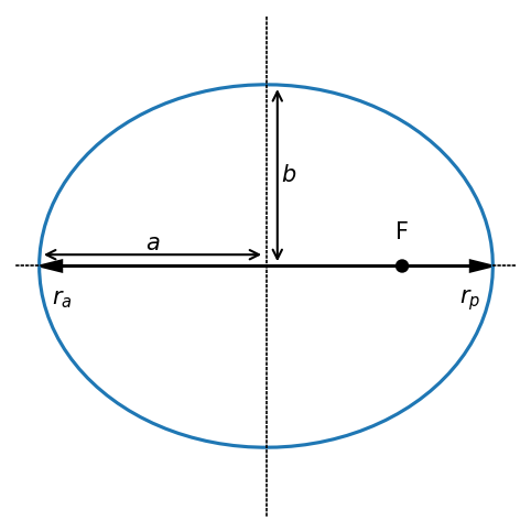
Some definitions:

focus: $F$, is the location of the center of mass of the body being orbited (e.g., Earth)
semi-major axis: $a$. This is also the average distance of the orbit.
semi-minor axis: $b$
point on the orbit nearest to the focus: periapse, with radial position $r_p$
point on the orbit furthest from the focus: apoapse, with radial position $r_a$
Apse line: the line connecting the focus and periapse.

For Earth-satellite systems, we call the periapse the perigee and the apoapse the apogee. These terms will vary depending on the body being orbited, for example in solar orbits we have the periapse and apoapse. The true anomaly $\theta$ starts at the apse line; $\theta = 0$ at periapse/perigee and $\theta = \pi$ at apoapse/apogee.

Some useful relationships:

\[\begin{split} \begin{align} a &= \frac{r_p + r_a}{2} \\ e &= \frac{r_a - r_p}{r_a + r_p} \\ r_p &= a (1-e) = \frac{h^2/\mu}{1 + e} \\ r_a &= a (1+e) = \frac{h^2/\mu}{1 - e} \\ h^2 &= a \mu (1 - e^2) \end{align} \end{split}\]

Example problem workflow¶

Problem: given the altitude of a satellite, the velocity magnitude $v_0$, flight-path angle $\gamma$, and knowing the gravitational parameter for an Earth-satellite system ($\mu$ = 398,600 km$^3$/s$^2$, find the eccentricity of the orbit $e$ and the true anomaly $\theta$.

Solution steps:

Find $r$ = altitude + $R_e = 6378 km (the average radius of the Earth).
Calculate the velocity components, then use $v_{\theta}$ to get the angular momentum:

\[\begin{split} \begin{align} v_r &= v_0 \sin \gamma = \frac{\mu}{h} e \sin \theta \\ v_{\theta} &= v_0 \cos \gamma = \frac{h}{r} \rightarrow h \end{align} \end{split}\]
Calculate $e \sin \theta$ and $e \cos \theta$:

\[\begin{split} \begin{align} v_0 \sin \gamma &= \frac{\mu}{h} e \sin \theta \rightarrow e \sin \theta \\ v_0 \cos \gamma = \frac{\mu}{h}(1 + e \cos \theta) \rightarrow e \cos \theta \end{align} \end{split}\]
Calculate the true anomaly $\theta$:

\[ \tan \theta = \frac{e \sin \theta}{e \cos \theta} \rightarrow \theta \]
Calculate the eccentricity:

\[ r = \frac{h^2/\mu}{1 + e \cos \theta} \rightarrow e \]

Warning

Altitude is not the same thing as the radial position! Altitude is measured from the surface of the Earth, so you need to add the Earth’s radius. (Also, this is not a constant value!)

Kepler’s Laws¶

We have already encountered Kepler’s first law! Originally, Brahe and Kepler though that orbits were circular, due to the mathematical/religious “perfection” of the shape. But, their predictions based on this idea did not match their (accurate) observations—they were always off.

Then, Kepler had an epiphany: an elliptical orbit would explain their observations.

Kepler’s First Law

Orbiting bodies travel in ellipses.

For Kepler’s second law, we need to look at how much time it takes orbits to sweep over a particular area:

\[\begin{split} \begin{align} v_{\theta} &= \frac{h}{r} \\ \rightarrow h &= r v_{\theta} = r \, r \, \dot{\theta} \\ h &= r^2 \frac{d\theta}{dt} \\ d\theta &= \frac{h}{r^2} dt \;, \end{align} \end{split}\]

but, we can also express a differential area as $dA = \frac{r^2}{2} d \theta$. Combining these together:

\[\begin{split} \begin{align} dA &= \frac{r^2}{2} d\theta = \frac{r^2}{2} \left( \frac{h}{r^2} dt \right) \\ \therefore \frac{dA}{dt} &= \frac{h}{2} \;, \end{align} \end{split}\]

which shows that the rate of change of area is constant! This is Kepler’s second law.

Kepler’s Second Law

Orbits sweep out equal areas in equal times.

We can obtain Kepler’s third law by integrating our result for area and time to find the orbital period:

\[\begin{split} \begin{align} \int dA &= \int \frac{h}{2} dt \\ \text{but } A &= a b \pi \quad b = a^2 (1 - e^2) \\ \rightarrow T &= \frac{2 \pi}{\sqrt{\mu}} a^{3/2} \;, \end{align} \end{split}\]

where $T$ is the period for an elliptic orbit.

Kepler’s Third Law

The square of the period of an elliptic is proportional to the cube of the mean distance (i.e., the semi-major axis): $T^2 \propto a^3$.

Hyperbolic orbits¶

Hyperbolic orbits occur for $e > 1$, and are known as flyby orbits because the object comes in close and fast to the central mass/focus. As the orbiting body moves away from the focus, off to infinity, the velocity asymptotically approaches a constant (as $r \rightarrow \infty$) excess velocity:

\[ v_{\infty} = \sqrt{\frac{\mu}{a}} \;. \]

We can also define the escape velocity, which is the velocity required at the perigee distance to achieve a hyperbolic orbit (and thus escape a stable, elliptical orbit):

\[ v_{\text{esc}} = \sqrt{ \frac{2 \mu}{r_p} } \;. \]

If the orbiting body has this velocity or higher at perigee, then it will escape in a hyperbolic orbit. If the velocity is less than this, then it will settle into a stable elliptic orbit.

Space Systems Engineering notes