# this line makes figures interactive in Jupyter notebooks
%matplotlib inline
from matplotlib import pyplot as plt
Notebook Cell
# these lines are only for helping improve the display
import matplotlib_inline.backend_inline
matplotlib_inline.backend_inline.set_matplotlib_formats('pdf', 'png')
plt.rcParams['figure.dpi']= 300
plt.rcParams['savefig.dpi'] = 300
plt.rcParams['mathtext.fontset'] = 'cm'
Single stage rocket

Figure 1:Single stage rocket, showing payload , propellant , and structure .
Figure 1 shows a single-stage rocket. The total mass of the vehicle at liftoff, also called the wet mass, is
where is the propellant mass, is the structural mass (also called the “inert mass” or “empty mass”), and is the payload mass. Then, the total mass at burnout, or the dry mass, is
The mass ratio of this rocket, the ratio of wet mass to dry mass, is then
which typically ranges 8 to 20. Mass ratio can also be expressed in terms of the component masses:
We can also define a number of other useful mass-related parameters. The payload ratio or payload fraction is the ratio of the payload to the initial vehicle mass (not including the payload itself):
The structural coefficient relates the structural/inert masses of the vehicle to the combined structural and propellant masses:
where lower indicates better structural efficiency of a vehicle. Components that contribute to include the skin, structure, propellant tank, pumps\slash piping, nozzle, etc.---all the components of the rocket that aren’t propellant or payload. While we generally want as small as possible, engineering considerations limit the minimum value in practice: .
We can express the mass ratio in terms of the payload ratio and structural coefficient:
and therefore we can also express in terms of these:
We can also define the propellant mass fraction, which is the fraction of the initial/wet mass that is propellant:
With a little work, we can show that the propellant mass fraction and rocket mass ratio are directly related:
Multistage rockets
Launch vehicles commonly use multiple stages, which each have their own propellant and inert/structure; the payload of one stage includes all upper stages. When the propellant of one stage is exhausted, that portion of the overall vehicle separates, reducing the overall structural mass. The purpose of staging rockets is essentially to achieve higher velocities, and/or more payload.
There are a few different styles of multiple-stage rockets, as Figure 2 shows for a few examples:
series/tandem: the booster, sustainer(s), and payload are stacked vertically
partial: droppable booster ring; sustainer includes propellant for the booster
parallel: boosters operating in parallel alongside sustainer
piggyback: various configurations, where sustainer stage(s) sit on the back of a booster.
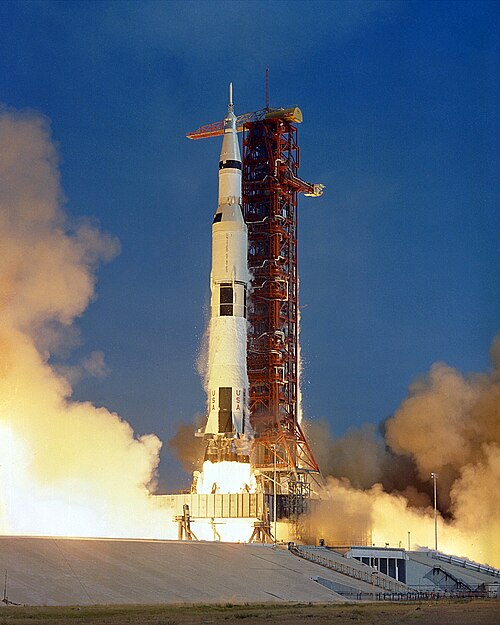
(a)Series/tandem staging: Saturn V
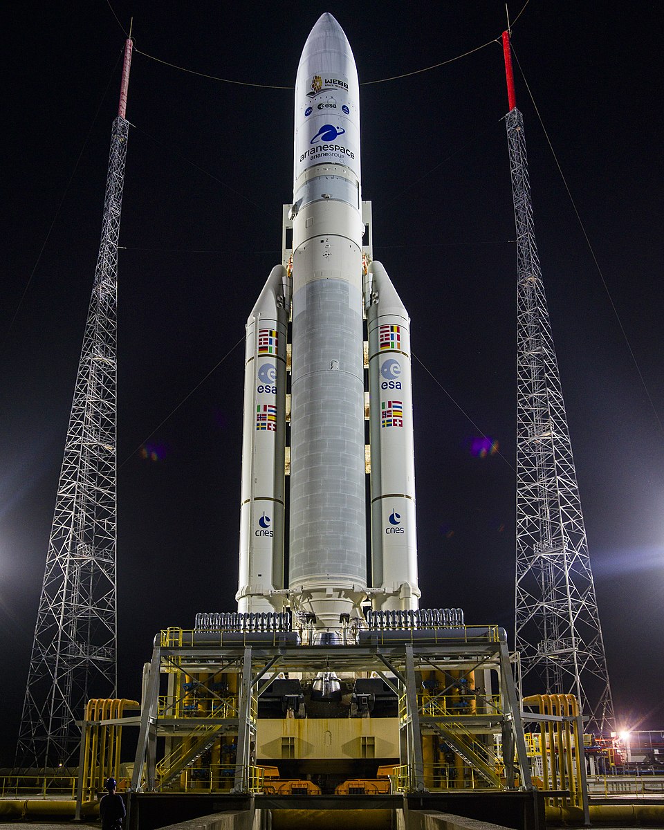
(b)Parallel staging: Ariane 5
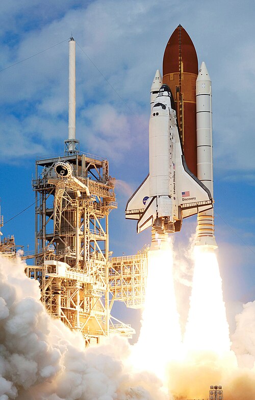
(c)Piggyback + parallel: Space Shuttle
Figure 2:Examples of common rocket staging styles. Sources: Saturn V, Ariane 5, Space Shuttle.
The series/tandem style is the most common, but all see regular use.
Let’s consider a three-stage series/tandem rocket, as shown in Figure 3.

Figure 3:Diagram of a three-stage rocket showing masses for each stage. Stage 1 (booster, on the bottom): , , total . Stage 2 (middle, sustainer): , , total . Stage 3 (top): , , , total .
Each stage has its own structural/inert and propellant masses; the payload of one stage includes all mass on the stages above it (including the actual vehicle payload at the top). The overall wet mass of the vehicle is the same as for the first stage:
and we can iteratively define the initial/wet and final/dry masses of each stage with respect to the next stage:
We can also define the nondimensional mass parameters for each stage :
and, for each stage, the mass ratio
and :
The overall for a vehicle with stages is then the sum of the contribution from each stage:
Similar stages
A rocket with similar stages shares a common effective exhaust velocity (meaning, common energetic performance and the same specific impulse ) and mass ratio MR for each stage:
and we can express the overall as
where is the number of stages.
It can be shown that similar stages is actually the optimal solution when each stage has the same energetic performance (constant ).
For a multistage rocket with similar stages, meaning each stage has the same effective exhaust velocity and structural ratio , the structural/empty mass and propellant mass for the th stage can be calculated:
where is the payload mass and is the payload fraction ().
The overall burnout velocity for an -stage similar-stage rocket is then
For an infinite number of stages, the burnout velocity would be
Example: varying number of stages
How does the achievable burnout velocity—which is the maximum for a launch vehicle—increase as the number of stages increases? How does this compare with the maximum theoretical velocity?
Determine for a multistage rocket with similar stages, each with , m/s, and an initial mass to payload mass ratio .
import numpy as np

struct_coeff = 0.2
eff_exhaust_velocity = 3000
m0_mPL = 30

payload_frac = 1. / m0_mPL
max_stages = 10

stages = list(range(1, max_stages + 1))
delta_v = np.zeros(max_stages)
mass_propellant_payload = np.zeros(max_stages)
for idx, N in enumerate(stages):
    delta_v[idx] = eff_exhaust_velocity * N * np.log(
        1 / (payload_frac**(1./N) * (1 - struct_coeff) + struct_coeff)
        )
    # ratio of stage propellant mass to payload
    for n in range(N):
        mass_propellant_payload[idx] += (
            (1 - payload_frac**(1./N))*(1 - struct_coeff) / payload_frac**((N - n)/N)
            )

delta_v_inf = eff_exhaust_velocity * (1 - struct_coeff) * np.log(1 / payload_frac)

fig, ax = plt.subplots()
ax.bar(stages, delta_v)
ax.set_xlabel('Number of stages')
ax.set_xticks(stages)
ax.set_ylabel('Burnout velocity (m/s)')
ax.axhline(delta_v_inf, ls='--')
ax.set_ylim([0, 10000])
ax.set_title(r'Total $\Delta V$ with number of stages')
plt.show()We can see that shifting from one stage to two and three stages gains a lot in terms of overall , but four or more stages has diminishing returns, even compared with the limiting result from an infinite number of stages.
What about propellant mass---how does the overall propellant mass compare for varying stages? To calculate this, we can use above for each stage, sum this up across all stages, and find the ratio of the total propellant mass to overall initial mass:
for idx, N in enumerate(stages):
    # ratio of stage propellant mass to payload
    mass_propellant_payload = 0.0
    for n in range(N):
        mass_propellant_payload += (
            (1 - payload_frac**(1./N))*(1 - struct_coeff) / payload_frac**((N - n)/N)
            )
    print(f'{N} stages: m_p / m_0 = {mass_propellant_payload * payload_frac: .2f}')
1 stages: m_p / m_0 = 0.77
2 stages: m_p / m_0 = 0.77
3 stages: m_p / m_0 = 0.77
4 stages: m_p / m_0 = 0.77
5 stages: m_p / m_0 = 0.77
6 stages: m_p / m_0 = 0.77
7 stages: m_p / m_0 = 0.77
8 stages: m_p / m_0 = 0.77
9 stages: m_p / m_0 = 0.77
10 stages: m_p / m_0 = 0.77
Interesting! With similar stages, the total amount of propellant is constant. However, the size of each stage will necessarily be different---the first stage is largest, and so on.
Let’s examine the amount of propellant in each stage, for both a single-stage and multiple-stage rockets.
mass_propellant_payload = np.zeros((max_stages,max_stages))
for idx, N in enumerate(stages):
    # ratio of stage propellant mass to payload
    for n in range(N):
        mass_propellant_payload[idx, n] = (
            (1 - payload_frac**(1./N))*(1 - struct_coeff) / payload_frac**((N - n)/N)
            )


fig, ax = plt.subplots()
im1 = ax.imshow(mass_propellant_payload * payload_frac,)
cb1 = fig.colorbar(im1, label=r'$m_p / m_0$')

ax.set_ylabel('Number of stages')
ax.set_xlabel('Stage number')
ax.set_title('Fraction of stage propellant mass to overall mass')

labels = [str(idx) for idx in range(1,max_stages+1)]

ax.set_xticks(range(max_stages), labels=labels)
ax.set_yticks(range(max_stages), labels=labels)

for (j,i),label in np.ndenumerate(mass_propellant_payload * payload_frac):
    if label > 0.0:
        if label > 0.5:
            color = 'black'
        else:
            color = 'white'
        ax.text(i,j,f'{label: .2f}',ha='center',va='center',c=color,fontsize='small')

plt.show()