Hybrid rockets combine elements of solid and liquid propulsion: a solid fuel grain with a liquid or gaseous oxidizer. The fuel and oxidizer are stored separately and only mix during combustion.
Motor Configuration
Figure 1:Schematic of a hybrid rocket motor showing: oxidizer tank (LOX or N₂O), oxidizer feed system with valve, injector, solid fuel grain with internal port(s), burning surface area , port area , and nozzle. The oxidizer flows through the port while fuel vaporizes from the grain surface.
Grain cross-sections:
Figure 2:Cross-section views of hybrid fuel grains: (a) Single cylindrical port — simplest configuration, (b) Multi-port (wagon wheel) — increases burning surface area relative to port area for higher thrust.
Common fuel materials:
HTPB — Hydroxyl-terminated polybutadiene:
Paraffin wax (high regression rate)
Other polymers and plastics
Combustion Physics
Unlike solid rockets (premixed combustion) or liquid rockets (rapid mixing), hybrids use non-premixed combustion with a diffusion flame.
Figure 3:Diffusion flame structure in a hybrid motor showing: oxidizer flow through the port, velocity boundary layer development along the fuel surface, flame zone where fuel vapor meets oxidizer, heat transfer back to fuel surface causing regression at rate , and fuel vapor rising from the surface.
The flame exists in a thin zone where:
Fuel vapor (from the grain surface) diffuses outward
Oxidizer diffuses inward from the core flow
They meet at stoichiometric proportions and combust
Advantages and Disadvantages
Advantages include:
Safety — Fuel and oxidizer do not mix prior to combustion; inert fuel grain
Throttleable — Adjust oxidizer flow rate to control thrust
Shutdown & restart — Simply stop/start oxidizer flow
Propellant versatility — More oxidizer options than solid motors
Environmentally cleaner — Products are mostly CO₂ and H₂O, vs. solids which produce HCl, Al₂O₃ (from AP/Al propellants)
Grain robustness — Less sensitive to cracks, voids, etc.
Lower temperature sensitivity — Performance less affected by ambient temperature
Disadvantages include:
Low regression rate (vs. solid) — Requires multi-port grains or long motors
Lower bulk density (vs. solid) — Less propellant per unit volume
Lower combustion efficiency: for hybrids, vs. for liquid engines
O/F shift — Mixture ratio changes during burn:
Fuel Regression Rate
Comparison to Solid Rockets
In a solid rocket motor (SRM), burning rate depends on chamber pressure:
In a hybrid motor, fuel regression rate depends on oxidizer mass flux:
where:
= oxidizer mass flux [kg/m²·s]
= oxidizer mass flow rate
= port cross-sectional area
Empirical Regression Rate Law
Figure 4:Log-log plot of fuel regression rate versus oxidizer mass flux . The slope of the line is the flux exponent . Different fuel materials have different and values.
Typical values:
| Parameter | Hybrid | Solid (for comparison) |
|---|---|---|
| 0.1 – 0.5 cm/s | ~1 in/s (2.5 cm/s) | |
| (0.05 – 0.2 mm/s) | ||
| 0.4 – 0.7 | 0.3 – 0.7 |
Mass Flow Rates
Total mass flow rate is:
where:
= oxidizer flow rate (controlled by feed system)
= fuel flow rate (determined by regression)
Figure 5:Fuel grain cross-section showing burning surface area , fuel density , and regression rate . The fuel mass flow is generated by surface regression.
The fuel mass flow rate is:
Substituting the regression rate law:
Circular Port Geometry
Figure 6:Cylindrical fuel grain with circular port of diameter (radius ) and length . Port area and burning surface area are shown.
For a circular port with radius and length :
Substituting into the fuel mass flow equation:
Equilibrium Chamber Pressure
Figure 7:Control volume for hybrid motor showing: oxidizer inflow , fuel addition from grain , chamber conditions (, , ), and nozzle outflow .
We can perform a control volume analysis to find an expression for the chamber pressure during a quasi-steady equilibrium operation. Applying mass conservation:
Using :
At quasi-steady state, we can approximate:
Substituting the fuel mass flow expression:
Solving for chamber pressure:
Given design requirements:
Choose target and ratio
Use CEA to determine
Select , geometry to satisfy the equilibrium equation
For circular port: ,
Time-Varying Behavior (O/F Shift)
Port Radius Evolution
As the fuel burns, the port radius increases with time.
For a circular port:
Substituting the regression rate law:
This is a separable ODE. Integrating:
where is the initial port radius.
Effect of Flux Exponent on Fuel Flow
Since :
The behavior of depends critically on the exponent :
| Condition | Behavior | Physical Interpretation |
|---|---|---|
| with time | Burning area grows faster than flux decreases | |
| with time | Flux decrease dominates | |
| constant | Effects balance |
Figure 8:Time evolution of fuel mass flow rate for different values of the flux exponent . Shows progressive (n < 0.5), neutral (n = 0.5), and regressive (n > 0.5) fuel flow behavior.
O/F Ratio Shift
Since is typically held constant (controlled by feed system) while varies:
The shifting O/F ratio affects:
(from thermochemistry)
(nozzle performance)
Therefore: and
import numpy as np
import matplotlib.pyplot as plt

from scipy.optimize import least_squares, root_scalar
from scipy.interpolate import UnivariateSpline

# Module used to parse and work with units
from pint import UnitRegistry
ureg = UnitRegistry()
Q_ = ureg.Quantity

# for convenience:
def to_si(quant):
    '''Converts a Pint Quantity to magnitude at base SI units.
    '''
    return quant.to_base_units().magnitude
Source
# these lines are only for helping improve the display
#import matplotlib_inline.backend_inline
#matplotlib_inline.backend_inline.set_matplotlib_formats('pdf', 'png')
plt.rcParams['figure.dpi']= 300
plt.rcParams['savefig.dpi'] = 300
plt.rcParams['mathtext.fontset'] = 'cm'
Extracting parameters
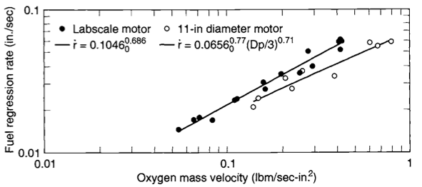
Figure 9:Experimental data and fits for HTPB/GOX fuel regression rate as a function of oxidizer mass flux. Source: Sutton & Biblarz (2016).
data = np.genfromtxt('hybrid-htpb-regression.csv', delimiter=',')def func(param, Go, rdot):
''' rdot = a * Go^n
'''
return rdot - param[0] * np.power(Go, param[1])res = least_squares(func, [0.1, 0.5], args=(data[:,0], data[:,1]))
print(res.x)[0.1058803 0.69835808]
plt.loglog(data[:,0], data[:,1], 'o')
Go = np.geomspace(0.05, 0.5, endpoint=True)
rdot = res.x[0] * np.power(Go, res.x[1])
plt.loglog(Go, rdot)
plt.show()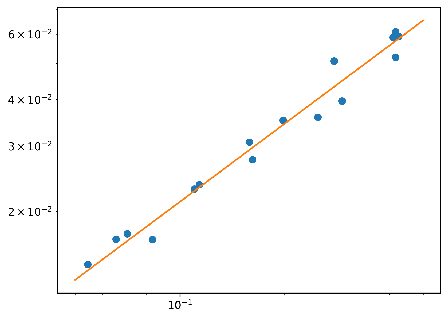
Design example
diameter_outer = Q_(1.175, 'in')

diameter_port = Q_(0.5, 'in')
diameter_throat = Q_(0.15, 'in')
length = Q_(10, 'in')
area_ratio = 5
density_fuel = Q_(915, 'kg/m^3')

vdot_ox = Q_(500, 'liter/min')
pressure_std = Q_(1, 'atm')
temperature_std = Q_(300, 'K')
gas_constant_air = Q_(8314, 'J/(kmol*K)') / Q_(32, 'kg/kmol')
# initial values
area_port = np.pi * diameter_port**2 / 4
area_burn = np.pi * diameter_port * length
mdot_ox = (pressure_std / (gas_constant_air * temperature_std)) * vdot_ox
print(f'Mass flow rate of oxidizer: {mdot_ox.to("kg/s"): .4f~P}')Mass flow rate of oxidizer: 0.0108 kg/s
volume_fuel = np.pi * length * ((diameter_outer/2)**2 - (diameter_port/2)**2)
mass_fuel_initial = density_fuel * volume_fuel

print(f'Initial fuel mass: {mass_fuel_initial.to("kg"):.2f~P}')
Initial fuel mass: 0.13 kg
Gox = (mdot_ox / area_port).to('lb/(s*in^2)')
rdot = Q_(0.104 * Gox.magnitude**0.681, 'in/s')
print(f'Fuel burning rate: {rdot: .4f~P}')
Fuel burning rate: 0.0248 in/s
mdot_fuel = density_fuel * area_burn * rdot
print(f'Mass flow rate of fuel: {mdot_fuel.to("kg/s"): .4f~P}')
Mass flow rate of fuel: 0.0058 kg/s
ox_fuel_ratio = mdot_ox / mdot_fuel
print(f'O/F ratio: {ox_fuel_ratio.to_base_units(): .3f~P}')
O/F ratio: 1.857
cstar = Q_(1759, 'm/s')
gamma = 1.1728
MW = Q_(20.828, 'g/mol')

area_throat = np.pi * diameter_throat**2 / 4

pressure_chamber = cstar * (mdot_ox + mdot_fuel) / area_throat
print(f'Chamber pressure: {pressure_chamber.to("psi"):.1f~P}')
Chamber pressure: 373.0 psi
def calc_thrust_coeff(gamma, pressure_ratio):
    ''' Calculates thrust coefficient for optimum expansion.
    pressure ratio: chamber / exit
    area ratio: exit / throat
    '''
    return np.sqrt(
        2 * np.power(gamma, 2) / (gamma - 1) *
        np.power(2 / (gamma + 1), (gamma + 1)/(gamma - 1)) *
        (1 - np.power(1.0 / pressure_ratio, (gamma - 1)/gamma))
        )

def calc_area_ratio(gamma, pressure_ratio):
    '''Calculates area ratio based on specific heat ratio and pressure ratio.
    pressure ratio: chamber / exit
    area ratio: exit / throat
    '''
    return (
        np.power(2 / (gamma + 1), 1/(gamma-1)) *
        np.power(pressure_ratio, 1 / gamma) *
        np.sqrt((gamma - 1) / (gamma + 1) /
                (1 - np.power(pressure_ratio, (1 - gamma)/gamma))
                )
        )

# This function returns zero for a given area ratio, pressure ratio, and gamma,
#and is used to numerically calculate pressure ratio given the other two values.
def root_area_ratio(pressure_ratio, gamma, area_ratio):
    ''' pressure ratio: chamber / exit
    area ratio: exit / throat
    '''
    return area_ratio - calc_area_ratio(gamma, pressure_ratio)
sol = root_scalar(root_area_ratio, x0=20, x1=100, args=(gamma, area_ratio))
pressure_ratio = sol.root
print(f'Pressure ratio: {pressure_ratio:.2f}')Pressure ratio: 29.57
thrust_coeff = calc_thrust_coeff(gamma, pressure_ratio)
print(f'Thrust coefficient: {thrust_coeff: .3f}')

specific_impulse = thrust_coeff * cstar / Q_(9.81, 'm/s^2')
thrust = thrust_coeff * pressure_chamber * area_throat

print(f'Specific impulse: {specific_impulse.to("s"): .1f~P}')
print(f'Thrust: {thrust.to("lbf"): .2f~P}')
Thrust coefficient: 1.485
Specific impulse: 266.3 s
Thrust: 9.79 lbf
oxid_fuel_ratios = np.arange(1.8, 5.3, 0.15)
gammas = []
cstars = []

with open('cea-output.txt', 'r') as f:
    lines = f.readlines()

for line in lines:
    if not line.strip():
        continue
    words = line.split()
    if words[0] == 'GAMMAs':
        gammas.append(float(words[2]))
    if words[0] == 'CSTAR,':
        cstars.append(float(words[2]))

gammas = np.array(gammas)
cstars = np.array(cstars)

assert len(oxid_fuel_ratios) == len(gammas)
assert len(oxid_fuel_ratios) == len(cstars)
cstar_fit = UnivariateSpline(oxid_fuel_ratios, cstars, s=0, ext='const')
gamma_fit = UnivariateSpline(oxid_fuel_ratios, gammas, s=0, ext='const')
fig, axes = plt.subplots(2, 1)
x = np.linspace(1.8, 5.5, 100)
axes[0].plot(oxid_fuel_ratios, cstars, 'o', label='From CEA')
axes[0].plot(x, cstar_fit(x), '--', label='Spline fit')
axes[0].set_ylabel(r'$c^*$ (m/s)')
axes[0].legend()
axes[0].grid(True)
axes[1].plot(oxid_fuel_ratios, gammas, 'o')
axes[1].plot(x, gamma_fit(x), '--')
axes[1].set_ylabel(r'$\gamma$')
axes[1].set_xlabel('O/F ratio')
axes[1].grid(True)
plt.show()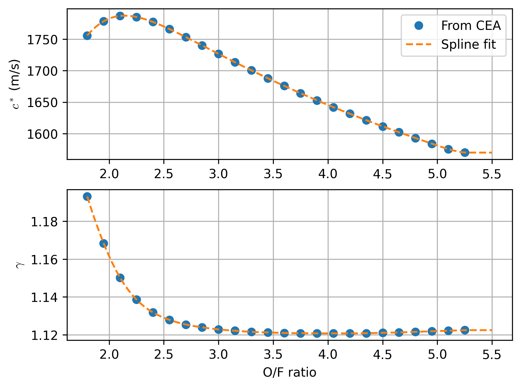
delta_t = Q_(1.0, 's')
times = Q_(np.arange(0.0, 101.0, 1), 's')

radii = Q_(np.zeros_like(times), 'in')
mdot_fuels = Q_(np.zeros_like(times), 'kg/s')
mixture_ratios = np.zeros_like(times)
specific_impulses = Q_(np.zeros_like(times), 's')
thrusts = Q_(np.zeros_like(times), 'lbf')

radius_initial = diameter_port / 2

for idx, time in enumerate(times):
    radii[idx] = Q_((
        (2*0.681 + 1)*0.104 * (mdot_ox.to('lb/s').magnitude / np.pi)**0.681 * time.to('s').magnitude +
        radius_initial.to('in').magnitude**(2*0.681 + 1)
        )**(1 / (2*0.681+1)),
        'in')

    area_port = np.pi * radii[idx]**2
    area_burn = np.pi * 2 * radii[idx] * length

    Gox = (mdot_ox / area_port).to('lb/(s*in^2)')
    rdot = Q_(0.104 * Gox.magnitude**0.681, 'in/s')
    mdot_fuels[idx] = density_fuel * area_burn * rdot
    mixture_ratios[idx] = mdot_ox / mdot_fuels[idx]

    cstar = Q_(cstar_fit(mixture_ratios[idx]), 'm/s')

    pressure_chamber = cstar * (mdot_ox + mdot_fuels[idx]) / area_throat

    specific_impulses[idx] = thrust_coeff * cstar / Q_(9.81, 'm/s^2')
    thrusts[idx] = thrust_coeff * pressure_chamber * area_throat

    # should stop when mass of fuel is exhausted
    mass_fuel_consumed = np.trapezoid(mdot_fuels, times)
    if mass_fuel_consumed >= mass_fuel_initial:
        idx_end = idx
        time_end = time
        print(f'Fuel exhausted at {time_end:.1f~P}')
        break
Fuel exhausted at 28.0 s
fig, axes = plt.subplots(2, 1)

axes[0].plot(times[:idx_end].magnitude, specific_impulses[:idx_end].to('s').magnitude)
axes[0].set_ylabel('Specific impulse (sec)')
axes[0].grid(True)

axes[1].plot(times[:idx_end].magnitude, thrusts[:idx_end].to('lbf').magnitude)
axes[1].set_ylabel('Thrust (lbf)')
axes[1].set_xlabel('Time (sec)')
axes[1].grid(True)

plt.show()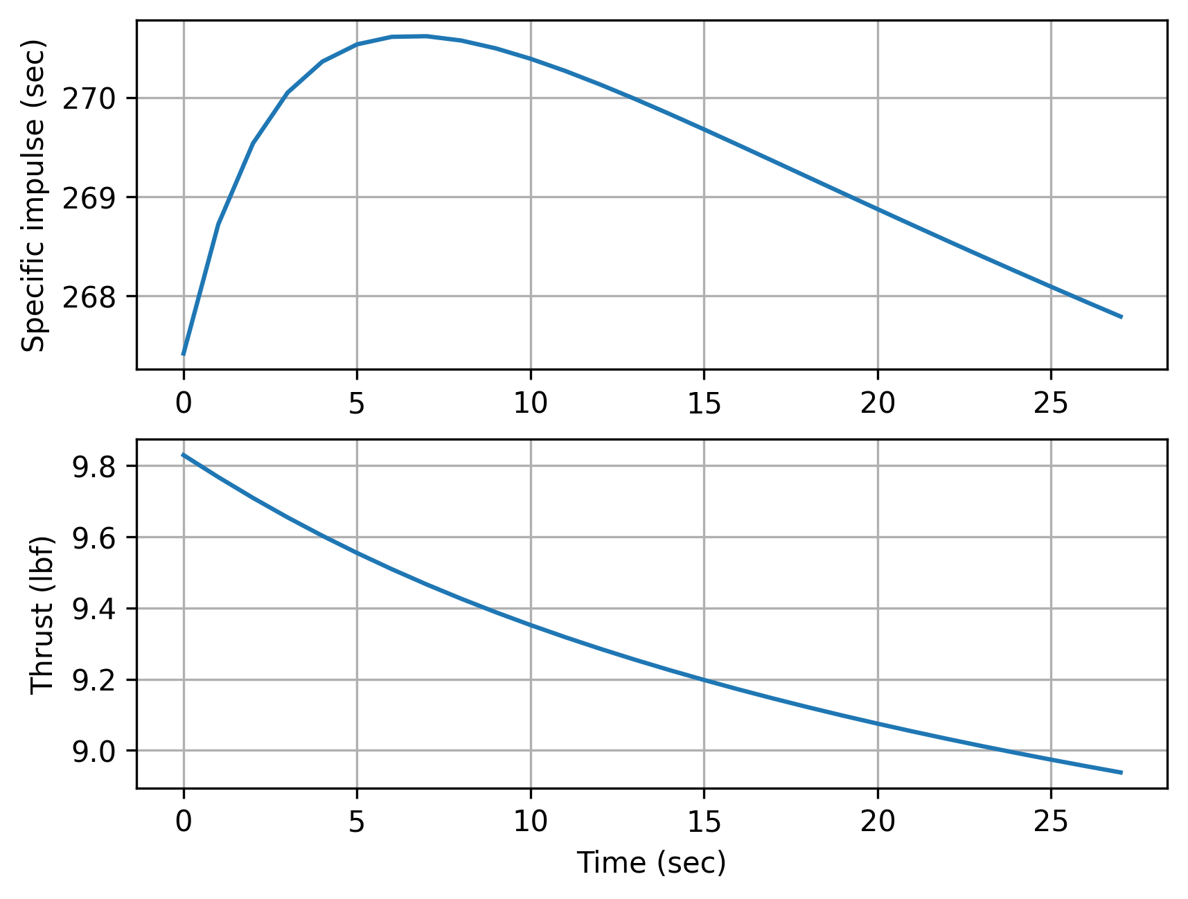
- Sutton, G. P., & Biblarz, O. (2016). Rocket Propulsion Elements (9th ed.). John Wiley & Sons.