Prandtl–Meyer flows - Gas Dynamics Notes

Prandtl–Meyer flows are isentropic turning flows that can involve compression or expansion. To describe them, we examine shocks at their weak limit.

Analysis of weak shocks¶

We can express the pressure change through a normal shock using Equation (143):

\begin{gather*} \frac{p_2}{p_1} = \frac{2\gamma}{\gamma+1} M_1^2 - \frac{\gamma-1}{\gamma+1} \\ \frac{p_2}{p_1} - 1 = \frac{\Delta p}{p_1} = \frac{2\gamma}{\gamma+1} (M_1^2 - 1) \;, \end{gather*}

(157)

so therefore through a normal shock $\Delta p \propto (M_1^2 - 1)$ .

We can also examine the entropy change through a normal shock by using one of our thermodynamic state relationships:

\begin{gather*} \Delta s_{1-2} = c_p \log \frac{v_2}{v_1} + c_v \log \frac{p_2}{p_1} \\ \frac{s_2 - s_1}{R} = \frac{\gamma}{\gamma-1} \log \frac{\rho_1}{\rho_2} + \frac{1}{\gamma-1} \log \frac{p_2}{p_1} \;, \end{gather*}

(158)

which, after considerable effort, we can express as

\frac{s_2 - s_1}{R} = \frac{2\gamma \left(M_1^2 - 1\right)^3}{3 (\gamma+1)^2} + \mathcal{O} \left( M_1^2 - 1 \right)^4 \;.

(159)

For weak shocks, where $M_1 \rightarrow 1$ , we can neglect the higher-order terms, and so $\Delta s \propto (M_1^2 - 1)^3$ .

For turning flows, the above analysis applies to the normal component of the Mach number: $M_{1n} = M_1 \sin \theta$ :

\frac{\Delta p}{p_1} = \frac{2\gamma}{\gamma+1} (M_1^2 \sin^2 \theta - 1)

(160)

and

\frac{\Delta s}{R} = \frac{2\gamma \left(M_1^2 \sin^2 \theta - 1\right)^3}{3 (\gamma+1)^2} + \mathcal{O} \left( M_1^2 \sin^2 \theta - 1 \right)^4 \;.

(161)

Small-angle approximations

We will use the small-angle approximations again. Recall that for small angles $\theta$ (in radians), we can approximate a right triangle with angle $\theta$ , base adjacent leg $A$ , opposite leg $O$ , and hypotenuse $H$ as the sector of a circle with radius $A$ and arc length $s$ . Then, $H \approx A$ , $O \approx s$ , and $s = A \theta$ .

Therefore, we can approximate:

\begin{gather*} \tan \theta = \frac{O}{A} \approx \frac{s}{A} = \frac{A \theta}{A} = \theta \;, \\ \sin \theta = \frac{O}{H} \approx \frac{O}{A} = \theta \;, \\ \cos \theta = \frac{A}{H} \approx 1 \;. \end{gather*}

(162)

For very weak oblique shocks, we can make specific approximations:

The deflection angle $\delta$ is very small ( $\delta \ll 1$ ), meaning we can use the small angle approximations to say $\tan \delta \approx \delta$ .
The shock angle $\theta$ approaches the Mach angle $\mu$ , where $\sin \mu = 1 / M$ .

Let’s apply these approximations to our oblique-shock relationship given by Equation (150):

\begin{gather*} \tan \delta = 2 \cot \theta \left[ \frac{M_1^2 \sin^2 \theta - 1}{M_1^2 (\gamma + \cos 2\theta) + 2} \right) \\ \rightarrow \delta \approx (\text{constants}) \left( M_1^2 \sin^2 \theta - 1 \right) \\ \delta \propto \left( M_1^2 \sin^2 \theta - 1 \right) \;, \end{gather*}

(163)

since $\mu$ is known for a given value of $M_1$ . Therefore, we can express the changes in pressure and entropy using the deflection angle:

\begin{gather*} \frac{\Delta p}{p_1} \approx \frac{2\gamma}{\gamma+1} (\text{constants}) \; \delta \\ \frac{\Delta s}{R} \approx \frac{2\gamma}{3 (\gamma+1)^2} \left[ (\text{constants}) \; \delta \right]^3 \end{gather*}

(164)

Now, we can say that for any weak oblique shock, for any initial conditions, that

\begin{gather*} \Delta p \propto \delta \phantom{\;.} \\ \Delta s \propto \delta^3 \;. \end{gather*}

(165)

Isentropic turns¶

So far we have been analyzing a single weak shock, which deflects the flow by an infinitesimal angle. Now, consider a flow undergoing a turn over a finite angle, but comprised of $n$ small turns.

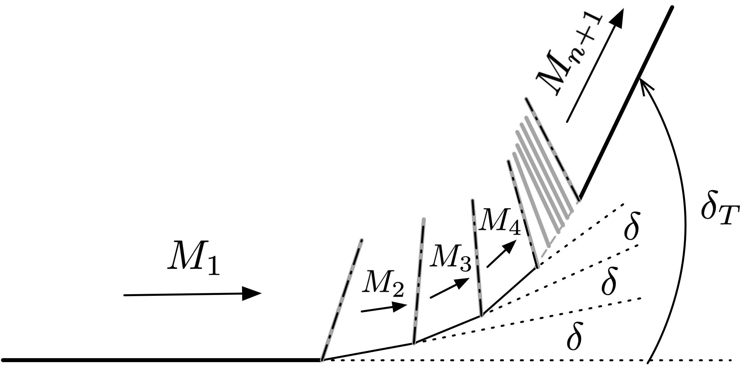
Diagram showing many small shock turns — Figure 4:A finite turning flow accomplished with many small turns from weak shocks.

With $n$ equal segments, the overall turning angle is $\delta_T = n \delta$ . For a given $\delta_T$ , increasing the number of segments $n$ will mean that each deflection $\delta$ decreases. Each segment is a very weak oblique shock, and for each $\Delta p^{\prime} \propto \delta$ and $\Delta s^{\prime} \propto \delta^3$ .

Then, if we look at the total change in pressure and entropy over the whole turn:

\begin{gather*} \Delta p = \sum^n \Delta p^{\prime} \propto n \, \delta \\ \Delta s = \sum^n \Delta s^{\prime} \propto n \, \delta^3 \;, \end{gather*}

(166)

but $\delta = \delta_T / n$ , so

\begin{gather*} \Delta p \propto \lim_{n \rightarrow \infty} n \left( \frac{\delta_T}{n} \right) = \delta_T \\ \Delta s \propto \lim_{n \rightarrow \infty} n \left( \frac{\delta_T}{n} \right)^3 = 0 \;. \end{gather*}

(167)

Therefore, as the number of segments increases and $n \rightarrow \infty$ ,

The wall makes a smooth turn through a finite angle $\delta_T$ ,
The shock waves become Mach waves,
The Mach number changes continuously,
There is a finite pressure change continuously through the turn, and
There is no change in entropy—the process is isentropic.

So, we can use smooth turns to achieve isentropic compression with a concave turn, and isentropic expansion with a convex turn—smooth or sharp.

Analysis of Prandtl-Meyer flows¶

Knowing that Prandtl-Meyer expansion/compression is isentropic, we want to know how the Mach number changes for a given turning angle: $\Delta M = f( \delta_T)$ . To derive this relationship, we can examine a single Mach wave to see how the flow changes instantaneously in an expansion fan.

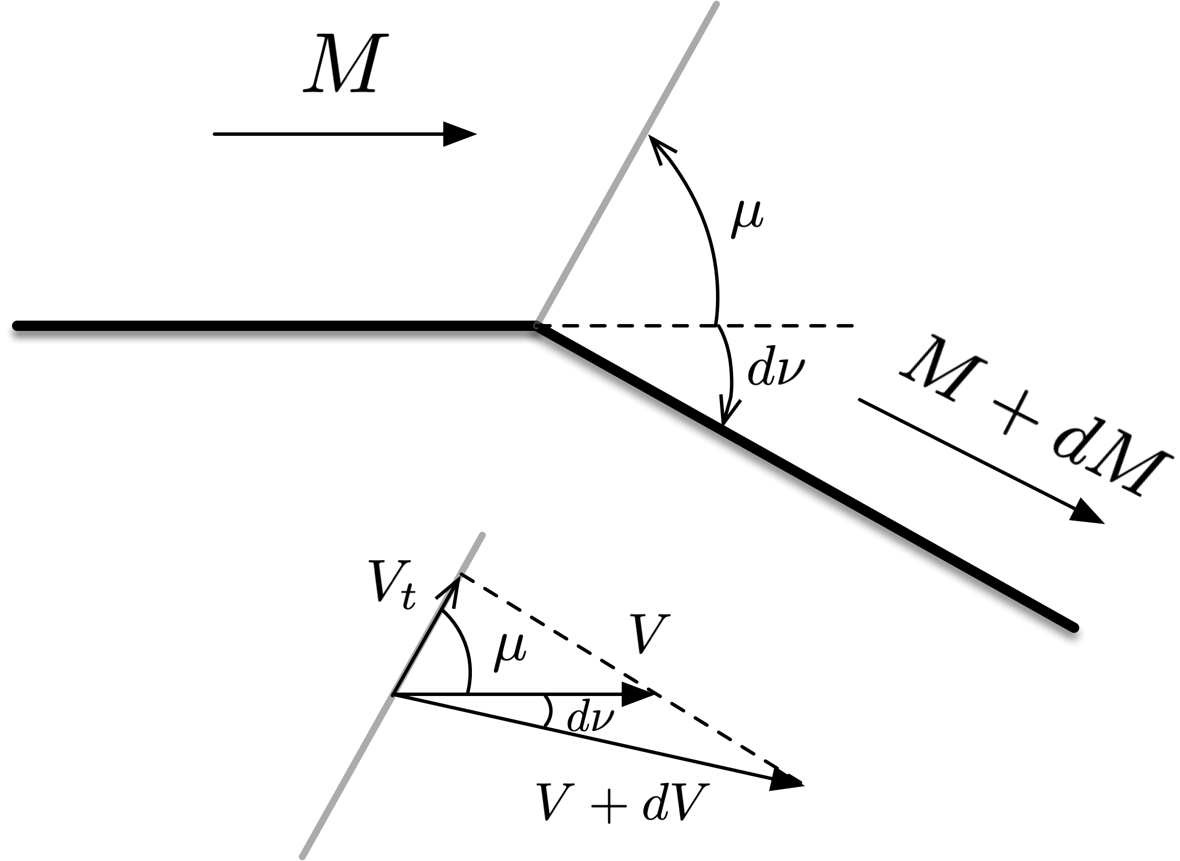
Diagram of flow change through a single Mach wave — Figure 5:Diagram of how flow changes through a single Mach wave in a Prandtl-Meyer expansion turn.

We start with a supersonic flow at Mach number $M$ , encountering a expansion Mach wave at angle $\mu$ . The flow turns through angle $d \nu$ and accelerates to $M + dM$ . Looking at the components of velocity, the tangential component $V_t$ does not change through the expansion wave:

\begin{gather*} V_t = V \cos \mu = (V + dV) \cos (\mu + d \nu) \\ V \cos \mu = (V + dV) \left( \cos \mu \cos d \nu - \sin \mu \sin d \nu \right) \end{gather*}

(168)

Since a single Mach wave will only turn the flow by an infinitesimal angle, we can apply the small-angle approximation: $d\nu \ll 1$ , so $\cos d \nu \approx 1$ and $\sin d\nu \approx d\nu$ . Therefore,

\begin{gather*} V \cos \mu = (V + dV) \left( \cos \mu - d\nu \sin \mu \right) \\ d \nu = \cot \mu \frac{dV}{V} \end{gather*}

(169)

But, since we have that $\sin \mu = \frac{1}{M}$ , we know that $\cos \mu = \sqrt{M^2 - 1}$ . Then,

\begin{gather*} d \nu = \sqrt{M^2 - 1} \frac{dV}{V} \\ \rightarrow d \nu = \frac{\sqrt{M^2 - 1}}{1 + \frac{\gamma-1}{2} M^2} \frac{dM}{M} \;. \end{gather*}

(170)

This gives us $d\nu = f(\gamma, M)$ , which we can integrate to get $\nu + \text{const} = f(\gamma, M)$ . If we specify the constraint that $\nu = 0$ for $M = 1$ , then the integration constant becomes zero, and the closed-form expression for $\nu$ is

\nu = \left( \frac{\gamma+1}{\gamma-1} \right)^{1/2} \tan^{-1} \left[ \frac{\gamma-1}{\gamma+1} \left( M^2 - 1 \right) \right]^{1/2} - \tan^{-1} \left( M^2 - 1\right)^{1/2} \;.

(171)

This is the Prandtl–Meyer function, the angle measured from the flow direction where $M = 1$ , through which a flow turned isentropically reaches $M$ .

If we know the downstream Mach number, we can solve Equation (171) easily to get the associated turning angle. Finding the new Mach number from the angle requires interpolation or numerical solution.

def get_prandtl_meyer(mach, gamma=1.4):
    '''Evaluate Prandtl-Meyer function at given Mach number.
    
    Defined as the angle from the flow direction where Mach = 1 through which the 
    flow turned isentropically reaches the specified Mach number.
    '''
    return (
        np.sqrt((gamma + 1) / (gamma - 1)) *
        np.arctan(np.sqrt((gamma - 1)*(mach**2 - 1)/(gamma + 1))) -
        np.arctan(np.sqrt(mach**2 - 1))
        )

def solve_prandtl_meyer(mach, nu, gamma=1.4):
    '''Solve for unknown Mach number, given Prandtl-Meyer function (in radians).'''
    return (nu - get_prandtl_meyer(mach, gamma))

Example: turn from sonic flow¶

Consider a horizontal airflow moving at $M = 1$ , which is turned 28° via a sharp corner. A centered Prandtl–Meyer expansion fan isentropically expands the flow. What is the final Mach number?

In this case, we can apply the Prandtl–Meyer function directly: $\nu$ = 28° from the flow direction where $M = 1$ . We can then solve for $M_2$ :

gamma = 1.4
turn_angle = 28 * np.pi/180

# guesses for M2: 2.0 and 3.0
root = root_scalar(solve_prandtl_meyer, x0=2.0, x1=3.0, args=(turn_angle, gamma))
print(f'M2 = {root.root: .3f}')

M2 =  2.059

Example: turn from general supersonic flow¶

Now, consider a horizontal airflow moving at a Mach number of 2.059, that encounters a sharp turn downward of 12°. What is the final Mach number?

We cannot just solve Equation (171) because the initial Mach number is not 1.0.

However, we can imagine that to obtain the true starting Mach number of 2.059, we hypothetically started with a flow at Mach = 1.0 and expanded it through a turn of 28°. Then, adding an additional 12° will reach the same final Mach number.

In other words, modify the problem such that $M_0 = 1 \rightarrow M_1 \rightarrow M_2$ , and $\nu_2 = \Delta \nu + \nu_1$ , where $\nu_1$ is the Prandtl–Meyer function evaluated at the actual starting Mach number $M_1$ , $\Delta \nu$ is the turning angle (12° in this case), and $\nu_2$ is the Prandtl–Meyer function of the final Mach number $M_2$ .

nu_1 = 28 * np.pi/180
delta_nu = 12 * np.pi/180

nu_2 = nu_1 + delta_nu
print(f'nu_2 = {nu_2*180/np.pi: .1f}°')

# guesses for M2: 2.0 and 3.0
root = root_scalar(solve_prandtl_meyer, x0=2.0, x1=3.0, args=(nu_2, gamma))
print(f'M_2 = {root.root: .3f}')

nu_2 =  40.0°
M_2 =  2.538

Therefore, for any Prandtl–Meyer flow, we can find the final Mach number from an arbitrary initial Mach number using

\nu_2 = \nu_1 + \Delta \nu \;,

(172)

where $\nu_1 = f(M_1, \gamma)$ , $\Delta \nu$ is the turning angle (positive for convex expanding flow, negative for concave compressing flow), and $\nu_2 = f(M_2, \gamma)$ .

Example: isentropic compression¶

Consider a Prandtl–Meyer compression problem: a horizontal airflow at Mach 2.40 encounters a smooth turn upward at 20°. What is the Mach number near the wall after the turn?

gamma = 1.4
M1 = 2.40

# turning angle is negative because compression
delta_nu = -20 * np.pi/180

nu_1 = get_prandtl_meyer(M1, gamma)
nu_2 = nu_1 + delta_nu

root = root_scalar(solve_prandtl_meyer, x0=1.5, x1=2.0, args=(nu_2, gamma))
print(f'M_2 = {root.root: .3f}')

M_2 =  1.664

However, what happens away from the wall? The flow needs to turn sharply, and an oblique shock forms with a deflection angle $\delta$ of 20°.

def oblique_shock_delta(theta, mach, gamma=1.4):
    '''Calculate oblique shock deflection from shock angle and Mach'''
    return (
        np.arctan((2.0/np.tan(theta)) * (
            (mach**2 * np.sin(theta)**2 - 1) /
            (2 + mach**2 * (gamma + np.cos(2*theta)))
            ))
        )

def solve_oblique_theta(theta, delta, mach, gamma=1.4):
    '''Solve for oblique wave angle theta'''
    return (delta - oblique_shock_delta(theta, mach, gamma))

def get_mach_normal(gamma, mach1):
    '''Calculate Mach number after a normal shock'''
    return np.sqrt(
        (mach1**2 + 2/(gamma - 1))/(2 * gamma * mach1**2/(gamma - 1) - 1)
        )

gamma = 1.4
M1 = 2.40
delta = 20 * np.pi/180

root = root_scalar(
    solve_oblique_theta, x0=40*np.pi/180, x1=50*np.pi/180,
    args=(delta, M1, gamma)
    )
theta = root.root
print(f'Theta: {theta * 180/np.pi: .2f}°')

M1n = M1 * np.sin(theta)
M2n = get_mach_normal(gamma, M1n)
M2 = M2n / np.sin(theta - delta)
print(f'M2: {M2: .3f}')

Theta:  44.34°
M2:  1.569

Due to the oblique shock, the Mach number away from the wall is lower than it is near the wall, and the pressure will be different too! So, there will need to be another wave phenomenon occuring between the two regions.