Flows with multiple effects - Gas Dynamics Notes

This module covers how we can analyze compressible flows with multiple effects accelerating or decelerating the flow: area change, friction, and/or heat transfer (plus shocks!).

Flows with friction and area change¶

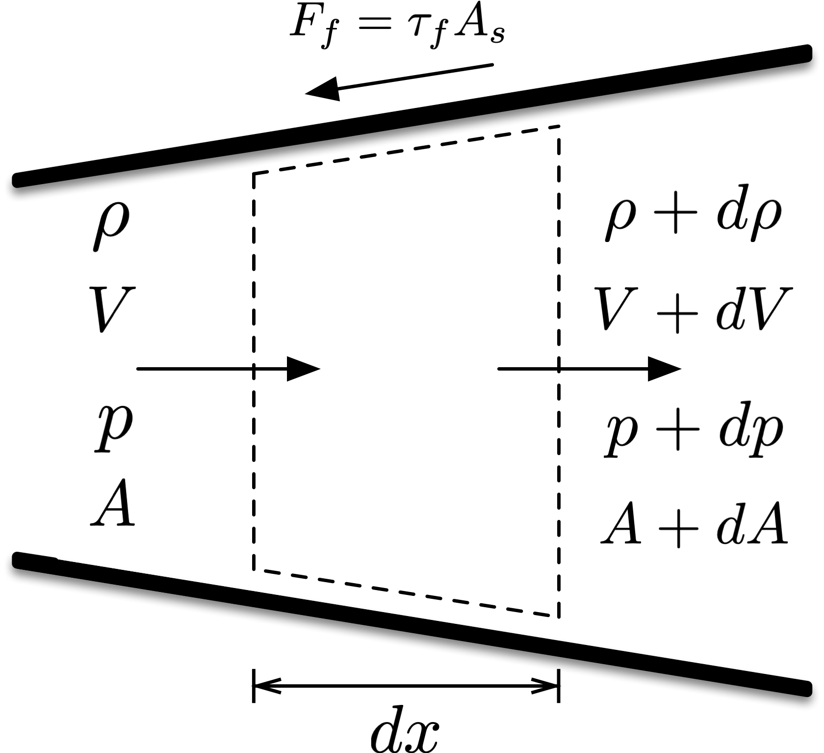
Control volume for flow with friction and area change — Figure 9:Differential control volume for adiabatic flow in a duct with varying area and friction.

Figure 9 shows a control volume in a varying-area duct, where the flow starts out with velocity $V$ , density $\rho$ , and pressure $p$ . The width of the differential control volume is $dx$ , the cross-sectional area of the duct is $A$ , and the wetted surface area is $A_s$ . The friction force $F_f$ is equivalent to the product of shear stress due to wall friction $\tau_f$ and $A_s$ .

First, we can apply conservation of mass to the control volume:

\begin{gather*} \rho V A = (\rho + d\rho) (V + dV) (A + dA) \\ 0 = \rho A dV + \rho V dA + A V d\rho \end{gather*}

(248)

0 = \frac{dV}{V} + \frac{dA}{A} + \frac{d\rho}{\rho}

(249)

Next, conservation of momentum:

\begin{gather*} \sum F_x = \dot{m} \left( V_{\text{out}, x} - V_{\text{in}, x} \right) \\ p A + \left( p + \frac{dp}{2} \right) dA - (p + dp) (A + dA) - \tau_f A_s = (\rho A V)(V + dV - V) \\ -A dp - \frac{1}{2} \rho V^2 \frac{f A_s}{4} = \rho A V dV \\ dp + \frac{1}{2} \rho V^2 \frac{f dx}{D} + \rho V dV = 0 \;, \end{gather*}

(250)

where $f \equiv 4 \tau_f / \left( \frac{1}{2} \rho V^2 \right)$ is the Darcy friction factor, and for a circular duct $A_s = \pi D dx = 4 A dx / D$ .

We can divide the entire expression by the ideal gas law $p = \rho R T$ (using $p$ p on the left-hand side and $\rho R T$ on the right-hand side), and incorporate the Mach number expression $V^2 = M^2 \gamma R T$ , or, expressed differently, $R T = V^2 / \left( M^2 \gamma \right)$ :

\frac{dp}{p} + \frac{1}{\rho R T} \frac{1}{2} \rho V^2 \frac{f dx}{D} + \frac{1}{\rho R T} \rho V dV = 0

(251)

\frac{dp}{p} + \frac{1}{2} \gamma M^2 \frac{f dx}{D} + \gamma M^2 \frac{dV}{V} = 0 \;.

(252)

Then, take the differential of the ideal gas law and divide that result by the ideal gas equation:

\begin{gather*} dp = R T d\rho + \rho R dT \\ \frac{dp}{p} = \frac{d\rho}{\rho} + \frac{dT}{T} \;, \end{gather*}

(253)

and insert that into Eq. (252) to get

\frac{d\rho}{\rho} + \frac{dT}{T} + \gamma M^2 \frac{dV}{V} + \frac{1}{2} \gamma M^2 \frac{f dx}{D} = 0 \;.

(254)

We can eliminate $d\rho / \rho$ using Equation (249):

- \left( \frac{dV}{V} + \frac{dA}{A} \right) + \frac{dT}{T} + \gamma M^2 \frac{dV}{V} + \frac{1}{2} \gamma M^2 \frac{f dx}{D} = 0 \;.

(255)

Next, let’s differentiate the Mach number expression for ideal gases:

\begin{gather*} V = M a = M \sqrt{\gamma R T} \\ dV = dM \sqrt{\gamma R T} + \frac{M \sqrt{\gamma R}}{2 \sqrt{T}} dT \\ \frac{dV}{V} = \frac{dM}{M} + \frac{1}{2} \frac{dT}{T} \;, \end{gather*}

(256)

which we can use to eliminate $dV / V$ . Finally, since the flow is adiabatic, we can use the fact that stagnation enthalpy remains constant:

\begin{gather*} T_t = \text{constant} = T \left( 1 + \frac{\gamma - 1}{2} M^2 \right) \\ \frac{dT}{T} + \frac{d \left( 1 + \frac{\gamma - 1}{2} M^2 \right)}{\left( 1 + \frac{\gamma - 1}{2} M^2 \right)} = 0 \\ \frac{dT}{T} = - \frac{ (\gamma - 1) M dM}{1 + \frac{\gamma - 1}{2} M^2} \;, \end{gather*}

(257)

which gives us an expression for $dT / T$ . Eliminating $dT / T$ and $dV / V$ leads to

\frac{1}{2} \gamma M^2 \frac{f dx}{D} = \frac{dA}{A} + \frac{2(1 - M^2)}{2 + (\gamma-1) M^2} \frac{dM}{M} \;.

(258)

Finally, we can divide by $dx$ , and obtain a differential equation that describes how Mach number changes in a compressible flow due to the effects of both area change (via $dA/dx$ ) and friction:

\frac{1}{2} \gamma M^2 \frac{f}{D} = \frac{1}{A} \frac{dA}{dx} + \frac{2 (1-M^2)}{M \left[ 2 + (\gamma-1) M^2 \right]} \frac{dM}{dx} \;.

(259)

Unfortunately, this is not something we can usually integrate analytically to get an exact solution (except for the specific cases of isentropic flow and constant-area Fanno flow). Instead, we’ll need to use integration methods to obtain numerical solutions.

First, let’s consider the cases where we do have exact solutions, so we can compare our numerical results, and then we will look at the general case of combined friction and varying-area effects.

Isentropic flow in converging nozzle¶

First, consider air flowing isentropically (and so $f = 0$ ) in a conically shaped converging nozzle, with length 10 cm, initial area of 50 cm $^2$ , outlet area of 40 cm $^2$ . The inflow temperature is 300 K and velocity is 100 m/s.

Find the outlet Mach number and compare against the exact solution.

For a conical nozzle, we can express the area using

A(x) = \frac{\pi}{4} D(x)^2 = \frac{\pi}{4} \left( D_i + \frac{D_o - D_i}{L} \right)^2

(260)

Then, the area term is

\frac{1}{A(x)} \frac{dA}{dx} = \frac{2}{D(x)} \frac{dD}{dx} = \frac{2 \frac{D_o - D_i}{L}}{D(x)} \;,

(261)

where the diameter is expressed as $D(x) = D_i + (D_o - D_i) \frac{x}{L}$ .

Substituting this into Equation (259), since $f = 0$ , we get

\frac{dM}{dx} = F(x,M) = - \left[ \frac{(D_o - D_i) / L}{D(x)} \right] \frac{2 + (\gamma-1)M^2}{1 - M^2} M \;,

(262)

which we can integrate over $x = [0, L]$ with the initial condition $M(x=0) = M_i = V_i / a_i$ .

gamma = 1.4
R = Q_(287, 'J/(kg*K)')
length = Q_(10, 'cm').to('m')
area_in = Q_(50, 'cm^2').to('m^2')
area_out = Q_(40, 'cm^2').to('m^2')

temperature_in = Q_(300, 'K')
velocity_in = Q_(100, 'm/s')

diameter_in = np.sqrt(area_in * 4 / np.pi)
diameter_out = np.sqrt(area_out * 4 / np.pi)

speed_sound_in = np.sqrt(gamma * R * temperature_in)
mach_in = (velocity_in / speed_sound_in).to_base_units()
print(f'M_in = {mach_in: .4f~P}')

M_in =  0.2880

def dMdx_isentropic(x, M, gamma, D_in, D_out, length):
    '''Equation for dM/dx in isentropic flow'''
    # conical nozzle
    diameter = D_in + (D_out - D_in) * x / length
    
    return (-M * ((D_out - D_in) / length / diameter) *
        ((2 + (gamma-1) * M**2) / (1 - M**2))
        )

# integrate from x = 0 to L, using maximum step size of 1 cm
sol = solve_ivp(
    dMdx_isentropic, [0, length.to('m').magnitude], [mach_in.magnitude], 
    max_step=0.01,
    args=(gamma, diameter_in.to('m').magnitude, 
          diameter_out.to('m').magnitude, length.to('m').magnitude
         )
    )

plt.plot(sol.t * 100, sol.y[0,:])

plt.ylim([0.28, 0.38])
plt.grid(True)
plt.ylabel('Mach number')
plt.xlabel('Distance (cm)')
plt.tight_layout()
#plt.savefig('isentropic-numerical.png')
plt.show()
plt.close()

Loading...

Next, we can compare this against the exact solution.

# compare against exact solution

mach_out = sol.y[0,-1]
print(f'M_out (numerical): {mach_out: .4f}')

def isentropic_area_ratio(mach2, mach1, area_ratio, gamma=1.4):
    '''Function for isentropic area ratio equation, solving for M2'''
    return (
        area_ratio - (mach1 / mach2) * (
            (1 + 0.5*(gamma-1)*mach2**2) / (1 + 0.5*(gamma-1)*mach1**2)
            )**((gamma+1) / (2*(gamma-1)))
        )

root = root_scalar(
    isentropic_area_ratio, x0=0.1, x1=0.5,
    args=(mach_in.magnitude, (area_out/area_in).to_base_units().magnitude, gamma)
    )
mach_out_exact = root.root
print(f'M_out (exact) = {mach_out_exact:.4f}')

print(f'Error: {100*np.abs(mach_out_exact-mach_out)/mach_out_exact: .3e} %')

M_out (numerical):  0.3719
M_out (exact) = 0.3719
Error:  1.206e-10 %

Subsonic flow with friction in constant area duct¶

Next, consider air flow in a constant area duct with friction. (This is Fanno flow.) The initial Mach number is $M_i = 0.6$ , the duct length is 45 cm, the diameter is 3 cm, and the friction factor is 0.02.

Find the outlet Mach number, and compare against the exact solution.

Since the area is constant, $\frac{dA}{dx} = 0$ , and Equation (259) simplifies to

\frac{dM}{dx} = F(x,M) = \frac{\gamma M^3 \left[ 2 + (\gamma-1) M^2 \right]}{4 (1-M^2)} \frac{f}{D} \;,

(263)

which we can integrate over $x = [0, L]$ with initial condition $M(x=0) = M_i$ .

gamma = 1.4
R = Q_(287, 'J/(kg*K)')
length = Q_(45, 'cm')
diameter = Q_(3, 'cm')
friction_factor = 0.02
mach_in = 0.60

def dMdx_fanno(x, M, gamma, f, D):
    '''Equation for dM/dx in Fanno flow'''    
    return (gamma * M**3 * (2 + (gamma-1)*M**2) * (f / D) /
        (4 * (1 - M**2))
        )

# integrate from x = 0 to L, using maximum step size of 3 cm
sol = solve_ivp(
    dMdx_fanno, [0, length.to('m').magnitude], [mach_in], 
    max_step=0.03,
    args=(gamma, friction_factor, diameter.to('m').magnitude)
    )

mach_out = sol.y[0,-1]

plt.plot(sol.t * 100, sol.y[0,:])

plt.ylim([0.60, 0.72])
plt.grid(True)
plt.ylabel('Mach number')
plt.xlabel('Distance (cm)')
plt.tight_layout()
#plt.savefig('numerical-fanno.png')
plt.show()
plt.close()

Loading...

We can compare this numerical solution to the exact solution for Fanno flow.

# compare with exact solution
print(f'M_out (numerical) = {mach_out: .4f}')

def fanno_distance(mach_2, mach_1, delta_x, friction, diameter, gamma=1.4):
    '''Function for Fanno flow, solving for M2'''
    return (
        (friction * delta_x / diameter) -  (((gamma+1)/(2*gamma)) *
            np.log((1 + 0.5*(gamma-1)*mach_2**2) / (1 + 0.5*(gamma-1)*mach_1**2)) -
            (1/gamma)*(1 / mach_2**2 - 1 / mach_1**2) -
            (gamma+1) * np.log(mach_2**2 / mach_1**2) / (2*gamma)
            )
        )

root = root_scalar(
    fanno_distance, x0=0.7, x1=0.8,
    args=(mach_in, length.to('m').magnitude, friction_factor, 
          diameter.to('m').magnitude, gamma)
          )
mach_out_exact = root.root
print(f'M_out (exact) = {mach_out_exact:.4f}')

print(f'Error: {100*np.abs(mach_out_exact-mach_out)/mach_out_exact: .4e} %')

M_out (numerical) =  0.7093
M_out (exact) = 0.7093
Error:  3.1377e-09 %

Flows with area change and friction¶

When the flow encounters both area change and friction, we need to solve the full version of Equation (259), rearranged for convenience:

\frac{dM}{dx} = F(x,M) = \left\{ \frac{M \left[ 2 + (\gamma - 1)M^2 \right]}{2} \right\} \left\{ \frac{ -\frac{1}{A} \frac{dA}{dx} + \frac{1}{2} \gamma M^2 \frac{f}{D}}{1 - M^2} \right\}

(264)

We can integrate this in theory, but if we want to analyze converging-diverging nozzles that are choked, as $M \rightarrow 1$ at some location, then $\frac{dM}{dx} \rightarrow \infty$ . So, we need some special treatment to handle this singularity.

The method of Beans (1970) uses l’Hôpital’s rule to get a finite value for $\frac{dM}{dx}$ as the Mach number approches one. To evaluate the derivative at this limit, we can take the derivative of the numerator and denominator at the limit, focusing on the term

\begin{align*} \lim_{M \rightarrow 1} \left[ \frac{-\frac{1}{A} \frac{dA}{dx} + \frac{1}{2} \gamma M^2 \frac{f}{D}}{1 - M^2} \right] &= \lim_{M \rightarrow 1} \left\{ \frac{\frac{d}{dx} \left( -\frac{1}{A} \frac{dA}{dx} + \frac{1}{2} \gamma M^2 \frac{f}{D} \right)}{-2 M \frac{dM}{dx}} \right\} \\ &= \frac{\frac{d}{dx} \left[ -\frac{1}{A} \left( \frac{dA}{dx} \right) \right]_{M \rightarrow 1} + \frac{1}{2} \gamma \frac{d}{dx} \left(\frac{f}{D} \right)_{M \rightarrow 1} + \gamma \left( \frac{f}{D} \right)_{M \rightarrow 1} \left( \frac{dM}{dx} \right)_{M \rightarrow 1}}{-2 \left( \frac{dM}{dx} \right)_{M \rightarrow 1}} \\ \end{align*}

(265)

Then, looking at the whole derivative as $M \rightarrow 1$ ,

\left( \frac{dM}{dx} \right)_{M \rightarrow 1} = \left( \frac{\gamma+1}{2} \right) \left\{ \frac{\frac{d}{dx} \left[ -\frac{1}{A} \left( \frac{dA}{dx} \right) \right]_{M \rightarrow 1} + \frac{1}{2} \gamma \frac{d}{dx} \left(\frac{f}{D} \right)_{M \rightarrow 1} + \gamma \left( \frac{f}{D} \right) \left( \frac{dM}{dx} \right)_{M \rightarrow 1}}{-2 \left( \frac{dM}{dx} \right)_{M \rightarrow 1}} \right\} \;,

(266)

which we can rearrange to get

\frac{4}{\gamma+1} \left( \frac{dM}{dx} \right)_{M \rightarrow 1}^2 + \gamma \left( \frac{f}{D} \right)_{M \rightarrow 1} \left( \frac{dM}{dx} \right)_{M \rightarrow 1} - \frac{d}{dx} \left( \frac{1}{A} \frac{dA}{dx} \right)_{M \rightarrow 1} + \frac{\gamma}{2}\frac{d}{dx} \left( \frac{f}{D} \right)_{M \rightarrow 1} = 0 \;.

(267)

This is a quadratic equation for the derivative $dM/dx$ as the Mach number approaches one. It has two roots at the sonic point, one negative and one positive:

$\frac{dM}{dx} > 0$ for accelerating flow, where $\frac{dA}{dx} < 0$ for subsonic flow and $\frac{dA}{dx} > 0$ for supersonic flow; and
$\frac{dM}{dx} < 0$ for decelerating flow, where $\frac{dA}{dx} > 0$ for subsonic flow and $\frac{dA}{dx} < 0$ for supersonic flow

Sonic location¶

To apply the appropriate solution, we need to find the location of the sonic point, found with

\left( -\frac{1}{A} \frac{dA}{dx} + \frac{1}{2} \gamma M^2 \frac{f}{D} \right)_{M \rightarrow 1} \rightarrow 0 \;.

(268)

To find the specific location, we need to consider a specific nozzle shape; let’s focus on a symmetrical nozzle with circular cross section, following the formula

D(x) = 2 \left[ 1 + \frac{1}{2} \cos \left( \pi \frac{x}{L} \right) \right] D_t \;,

(269)

where the diameter is $3 D_t$ at $x = 0$ , $D_t$ at $x=L$ , and $3 D_t$ at $x = 2L$ . For a circular nozzle, $\frac{1}{A} \frac{dA}{dx} = \frac{2}{D} \frac{dD}{dx}$ .

Applying the specifics of this nozzle to Equation (268):

\begin{gather*} \left( \frac{2}{D} \frac{dD}{dx} \right)_{M \rightarrow 1} = \left( \frac{\gamma}{2} \frac{f}{D} \right)_{M \rightarrow 1} \\ \left[ \frac{2}{D(x)} \frac{-\pi D_t}{L} \sin \left( \frac{\pi x}{L} \right) \right]_{M \rightarrow 1} = \left( \frac{\gamma}{2} \frac{f}{D(x)} \right)_{M \rightarrow 1} \\ \sin \left( \frac{\pi x_{\text{sp}}}{L} \right) = - \frac{\gamma f L}{4 \pi D_t} \\ \left( \frac{x}{L} \right)_{\text{sp}} = - \frac{1}{\pi} \sin^{-1} \left( \frac{\gamma f L}{4 \pi D_t} \right) \end{gather*}

(270)

For a case where $\gamma = 1.4$ , $f = 0.4$ , and $L = 2 D_t$ , we can calculate the sonic location:

gamma = 1.4
f = 0.4
angle = np.arcsin(gamma * f * 2 / (4*np.pi))
if angle < np.pi:
    angle = angle + np.pi
x_L_sp = (1/np.pi) * angle
print(f'(x/L) @ sonic = {x_L_sp: .4f}')

(x/L) @ sonic =  1.0284

(This does require some careful calculation to get the right value.)

Now, with the sonic location identified, calculating the Mach number distribution throughout the nozzle requires solving two initial value problems: from the sonic point backwards to the inlet, and from the sonic point forwards to the outlet. For points at/near the sonic point, we can use Equation (267) to find $dM/dx$ .

Let’s continue the case from before: air flowing through a symmetrical converging-diverging nozzle with a circular cross section, with the diameter given by Equation (269). The nozzle length is $L = 2 D_t$ and friction factor is $f = 0.4$ (this is very large).

# for solving quadratic equation at M = 1
Dsp = 2*(1 + 0.5*np.cos(np.pi*x_L_sp)) # * Dt
dD_dx_sp = -np.pi * np.sin(np.pi * x_L_sp) # *Dt/L
d2D_dx2_sp = -np.pi**2 * np.cos(np.pi * x_L_sp) # * Dt/L^2

a = 4 / (gamma + 1)
b = 2 * gamma * f / Dsp
c = -2*d2D_dx2_sp/Dsp + 2*(dD_dx_sp/Dsp)**2 - 2*gamma*f*dD_dx_sp/(2*Dsp**2)

# dM/d(x/L) at sonic point
roots = np.roots([a, b, c])
# take the positive root for accelerating flow
dM_dxL_sp = np.max(roots)

def area_function(x_L):
    '''Function for (1/A)*(dA/dx) using x/L'''
    return (-np.pi * np.sin(np.pi * x_L) / 
            (1 + 0.5 * np.cos(np.pi * x_L))
        )

def diameter_function(x_L):
    '''Function for nondimensional D'''
    return (1 + 0.5*np.cos(np.pi * x_L))

def dMdx_friction_area(x_L, M, gamma, area_func, f, diameter_func, dM_dxL_sp):
    '''dM/dx for flows with friction and area change.
    
    area_func is a function for (1/A)*(dA/dx)
    '''
    # when in neighborhood of M = 1, use special version of dM/dx
    if np.abs(M - 1) < 0.01:
        return dM_dxL_sp
    else:
        return (
            0.5*M*(2 + (gamma-1)*M**2) * (
                -area_func(x_L) + 0.5*gamma*M**2 * f/diameter_func(x_L)
                ) / (1 - M**2)
            )

# integrate x/L from sonic point to 0
x_vals = np.hstack(([x_L_sp], np.arange(1, 0, -0.05), [0]))

sol_sub = solve_ivp(
    dMdx_friction_area, [x_L_sp, 0], [1.0], 
    t_eval=x_vals,
    args=(gamma, area_function, f, diameter_function, dM_dxL_sp)
    )

# integrate x/L from sonic point to 2
x_vals = np.hstack(([x_L_sp], np.arange(1.05, 2.05, 0.05)))

sol_super = solve_ivp(
    dMdx_friction_area, [x_vals[0], x_vals[-1]], [1.0], 
    t_eval=x_vals,
    args=(gamma, area_function, f, diameter_function, dM_dxL_sp)
    )

# compare with isentropic
f = 0
x_L_sp = 1.0

# for solving quadratic equation at M = 1
Dsp = 2*(1 + 0.5*np.cos(np.pi*x_L_sp)) # * Dt
dD_dx_sp = -np.pi * np.sin(np.pi * x_L_sp) # *Dt/L
d2D_dx2_sp = -np.pi**2 * np.cos(np.pi * x_L_sp) # * Dt/L^2

a = 4 / (gamma + 1)
b = 2 * gamma * f / Dsp
c = -2*d2D_dx2_sp/Dsp + 2*(dD_dx_sp/Dsp)**2 - 2*gamma*f*dD_dx_sp/(2*Dsp**2)

# dM/d(x/L) at sonic point
roots = np.roots([a, b, c])
# take the positive root for accelerating flow
dM_dxL_sp = np.max(roots)


# integrate x/L from sonic point to 0
x_vals = np.hstack((np.arange(1, 0, -0.05), [0]))

sol_sub_isen = solve_ivp(
    dMdx_friction_area, [x_L_sp, 0], [1.0], 
    t_eval=x_vals,
    args=(gamma, area_function, f, diameter_function, dM_dxL_sp)
    )

# integrate x/L from sonic point to 2
x_vals = np.arange(1.0, 2.05, 0.05)

sol_super_isen = solve_ivp(
    dMdx_friction_area, [x_vals[0], x_vals[-1]], [1.0], 
    t_eval=x_vals,
    args=(gamma, area_function, f, diameter_function, dM_dxL_sp)
    )

plt.plot(
    np.hstack((sol_sub.t[::-1], sol_super.t)), 
    np.hstack((sol_sub.y[0,::-1], sol_super.y[0,:])), label='with friction'
    )

plt.plot(
    np.hstack((sol_sub_isen.t[::-1], sol_super_isen.t)), 
    np.hstack((sol_sub_isen.y[0,::-1], sol_super_isen.y[0,:])), '--', label='isentropic'
    )

plt.xlabel(r'$x / L$')
plt.ylabel('Mach number')
plt.grid(True)
plt.legend()
plt.tight_layout()
#plt.savefig('area-friction.png')
plt.show()
plt.close()

Loading...

We can see that the presence of friction starts to significantly alter the flow in the supersonic region, decelerating the flow from the isentropic solution and even causing the Mach number to begin decreasing near the exit. This is an extreme case, due to the high friction factor.

Computing other properties¶

Once we’ve solved for the distribution of Mach number in a flow system, we may want to obtain other properties such as pressure, temperature, and density. Since we cannot use the isentropic or Fanno flow relations, we need to derive new ones that apply under the current conditions where both area change and friction affect the flow.

For a more-general one-dimensional flow, conservation of mass applies, and we can use ideal-gas relationships:

\begin{gather*} \dot{m} = \rho A V = \text{constant} \\ V = M a = M \sqrt{\gamma R T} \\ p = \rho R T \end{gather*}

(271)

For an adiabatic flow, we also have that stagnation temperature is constant, and we can relate that to the static temperature using the appropriate stagnation relationship:

T_t = T \left( 1 + \frac{\gamma-1}{2} M^2 \right) \;.

(272)

Between two points $i$ and $j$ in the flow system (at locations $x_i$ and $x_j$ ), we can then write that $(T_t)_i = (T_t)_j$ , and if we know $M(x)$ , then

\frac{T_j}{T_i} = \frac{2 + (\gamma-1) M_i^2}{2 + (\gamma-1) M_j^2} \;.

(273)

Then, applying conservation of mass between those same two points:

\begin{gather*} \left( \rho A V \right)_i = \left( \rho A V \right)_j \\ \left( \frac{p}{RT} A M \sqrt{\gamma R T} \right)_i = \left( \frac{p}{RT} A M \sqrt{\gamma R T} \right)_j \end{gather*}

(274)

\frac{p_j}{p_i} = \frac{A_i}{A_j} \frac{M_i}{M_j} \sqrt{ \frac{T_j}{T_i} } \;,

(275)

and if we incorporate the temperature relationship from Equation (273) we can get

\frac{p_j}{p_i} = \frac{A_i}{A_j} \frac{M_i}{M_j} \left[ \frac{2 + (\gamma-1) M_i^2}{2 + (\gamma-1) M_j^2} \right]^{1/2} \;.

(276)

Similarly, for density we can arrive at a similar expression:

\frac{\rho_j}{\rho_i} = \frac{A_i}{A_j} \frac{M_i}{M_j} \sqrt{\frac{T_i}{T_j}} = \frac{A_i}{A_j} \frac{M_i}{M_j} \left[ \frac{2 + (\gamma-1) M_j^2}{2 + (\gamma-1) M_i^2} \right]^{1/2} \;.

(277)

Flows with heat transfer and area change¶

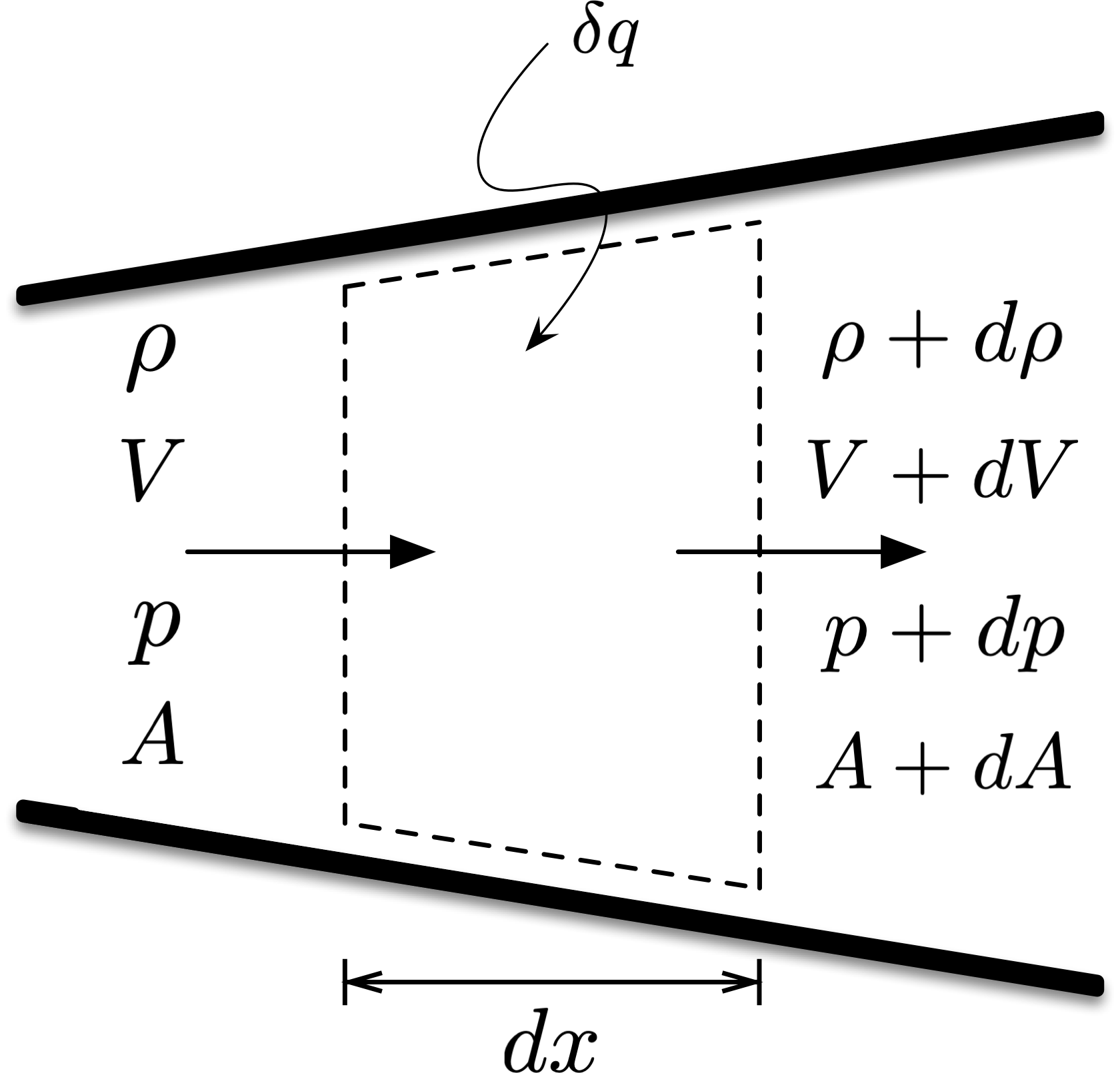
Control volume for flow with heat transfer and area change — Figure 10:Differential control volume for frictionless flow in a duct with varying area and heat transfer.

Figure 10 shows a control volume in a varying-area duct, where the flow starts out with velocity $V$ , density $\rho$ , and pressure $p$ . The width of the differential control volume is $dx$ , the cross-sectional area of the duct is $A$ , and the flow experiences heat transfer $\delta q$ .

Applying conservation of mass, momentum, and energy to the control volume, we get

\frac{d\rho}{\rho} + \frac{dA}{A} + \frac{dV}{V} = 0

(278)

dp + \rho V dV = 0

(279)

\delta q = c_p d T_t \;,

(280)

and we also can express a differential form of the ideal gas law:

\frac{dp}{p} = \frac{d\rho}{\rho} + \frac{dT}{T}

(281)

We can eliminate $\frac{dp}{p}$ by taking Equation (279) and dividing by $p$ , where we get

\begin{gather*} \frac{dp}{p} + \frac{\rho}{p} V dV = 0 \\ \rightarrow \frac{d\rho}{\rho} + \frac{dT}{T} + \frac{\rho}{p} V dV = 0 \;. \end{gather*}

(282)

Next, incorporate Equation (278) to eliminate $\frac{d\rho}{\rho}$ and use the ideal gas law expression

\frac{\rho}{p} V dV = \frac{\rho}{p} V^2 \frac{dV}{V} = \frac{1}{RT} M^2 \gamma R T \frac{dV}{V} = \gamma M^2 \frac{dV}{V}

(283)

to get

- \left( \frac{dA}{A} + \frac{dV}{V} \right) + \frac{dT}{T} + \gamma M^2 \frac{dV}{V} = 0 \;.

(284)

We can use the logarithmic derivative of the Mach number expression to eliminate $\frac{dV}{V}$ :

\begin{gather*} V = M \sqrt{ \gamma R T } \\ dV = dM \sqrt{\gamma R T} + dT \frac{1}{2} \frac{1}{\sqrt{T}} M \sqrt{\gamma R} \\ \frac{dV}{V} = \frac{dM}{M} + \frac{1}{2} \frac{dT}{T} \end{gather*}

(285)

and get

-\frac{dA}{A} + \frac{dM}{M} \left(\gamma M^2 - 1 \right) + \frac{dT}{T} \left( \frac{\gamma M^2 + 1}{2} \right) = 0 \;.

(286)

To eliminate $\frac{dT}{T}$ , we can look at the stagnation temperature relationship:

\begin{gather*} T_t = T \left( 1 + \frac{\gamma-1}{2} M^2 \right) \\ dT_t = dT \left( 1 + \frac{\gamma-1}{2} M^2 \right) + T (\gamma-1) M dM \\ \frac{dT_t}{T} = \left( 1 + \frac{\gamma-1}{2} M^2 \right) \frac{dT}{T} + (\gamma-1) M^2 \frac{dM}{M} \;, \end{gather*}

(287)

but we have from Equation (280) that $dT_t = \delta q / c_p$ , so

\frac{dT}{T} = \left( 1 + \frac{\gamma-1}{2} M^2 \right)^{-1} \left[ \frac{\delta q}{c_p T} - M^2 (\gamma-1) \frac{dM}{M} \right] \;,

(288)

which we can substitute into the above expression to get

-\frac{dA}{A} + \frac{ \gamma M^2 + 1}{2 \left( 1 + \frac{\gamma-1}{2} M^2 \right)} \frac{\delta q}{c_p T} + \frac{M^2 - 1}{1 + \frac{\gamma-1}{2} M^2} \frac{dM}{M} = 0 \;.

(289)

Rearranging and dividing by $dx$ , we can get an ordinary differential equation for solving for Mach number:

\frac{dM}{dx} = \frac{M}{1 - M^2} \left[ -\left(1 + \frac{\gamma-1}{2} M^2 \right) \frac{1}{A} \frac{dA}{dx} + \frac{1 + \gamma M^2}{2} \left( \frac{1}{c_p T} \frac{\delta q}{dx} \right) \right]

(290)

To integrate $M(x)$ , we need to know how the area changes with position and the rate that heat transfer occurs with distance.

Example: heat transfer in coverging nozzle with shock¶

As an example, consider air flow in a diverging conical nozzle of length 10 cm, where the diameter grows linearly with distance from 2 cm to 5 cm. The air enters the nozzle at a Mach number of 3 with a stagnation temperature of 300 K. Heat is added at a rate such that $\frac{dT_t}{dx}$ = 100 K/m. Due to the pressure at the exit, there is a normal shock wave halfway down the nozzle.

Thanks to our relationship between heat transfer and stagnation temperature, $\delta q = c_p d T_t$ , and our prior stagnation relationship for temperature, we can rewrite Equation (290) for this problem:

\frac{dM}{dx} = \frac{M \left[ 2 + (\gamma-1) M^2 \right]}{2 (1-M^2)} \left[ -\frac{1}{A} \frac{dA}{dx} + \frac{1+\gamma M^2}{2} \left( \frac{1}{T_t} \frac{dT_t}{dt} \right) \right] \;.

(291)

The nozzle diameter varies linearly with length:

D(x) = D_i + (D_e - D_i) \frac{x}{L} \;,

(292)

and so we can express the area and rate of change of area as

\begin{gather*} A(x) = \frac{\pi}{4} D(x)^2 = \frac{\pi}{4} \left[ D_i + (D_e - D_i) \frac{x}{L} \right]^2 \\ \rightarrow \frac{1}{A(x)} \frac{dA}{dx} = \frac{2}{D(x)} \frac{dD}{dx} = 2 \frac{\frac{D_e-D_i}{L}}{D(x)} = \frac{2 \alpha}{D(x} \end{gather*}

(293)

where $\alpha = (D_e - D_i) / L = 0.3$ and $D(x) = D_i + \alpha x$ . This leads to a specific $dM / dx$ for this problem:

\frac{dM}{dx} = \frac{M \left[ 2 + (\gamma-1) M^2 \right]}{2(1-M^2)} \left[ - \left( \frac{2\alpha}{D_i + \alpha x} \right) + \left( \frac{1 + \gamma M^2}{2} \right) \left( \frac{\beta}{(T_t)_i + \beta x} \right) \right]

(294)

and we can write a function that evaluates this:

def dMdx_heat_area(x, M, gamma, alpha, beta, D_in, Tt_in):
    '''Returns dM/dx for nozzle with heat transfer and area change'''
    return (
        0.5 * M * (2 + (gamma-1)*M**2) / (1 - M**2) * (
            -2*alpha/(D_in + alpha*x) + 
            0.5*(1+gamma*M**2) * beta / (Tt_in + beta*x)
            )
        )

We also need to handle the normal shock wave at the middle of the nozzle. The shock is a discontinuity at $x = 0.5 L$ , and so we can only integrate for $M(x)$ from $x = [0, 0.5 L]$ before we need to account for the shock by using our normal shock relationship. Then, using the new Mach number following the shock, we can continue the integration over $x = [0.5 L, L]$ .

For comparison, we can also calculate the adiabatic flow solution, which is isentropic except for the normal shock.

def normal_shock(mach, gamma=1.4):
    '''Returns Mach number after normal shock wave'''
    return np.sqrt(
        (mach**2 + 2/(gamma-1)) / (2*gamma*mach**2/(gamma-1) - 1)
        )

# problem parameters
mach_in = 3.0
gamma = 1.4

diam_in = Q_(2, 'cm').to('m')
diam_exit = Q_(5, 'cm').to('m')
length = Q_(10, 'cm').to('m')
alpha = ((diam_exit - diam_in) / length).to_base_units().magnitude

# shock location: x = 5 cm
stag_temp_in = 300
beta = 100 # K/m

# first solve to shock over x = [0, 0.5 L]:
sol_1 = solve_ivp(
    dMdx_heat_area, [0, length.magnitude / 2], [mach_in],
    max_step = 0.001,
    args=(gamma, alpha, beta, diam_in.magnitude, stag_temp_in)
    )

# find the Mach number after the normal shock
mach_post_shock = normal_shock(sol_1.y[0,-1], gamma)

# complete the integration over x = [0.5 L, L]:
sol_2 = solve_ivp(
    dMdx_heat_area, [length.magnitude / 2, length.magnitude], [mach_post_shock],
    max_step = 0.001,
    args=(gamma, alpha, beta, diam_in.magnitude, stag_temp_in)
    )

# adiabatic solution: isentropic except for the shock
# first solve to shock over x = [0, 0.5 L]:
sol_1_adiabatic = solve_ivp(
    dMdx_heat_area, [0, length.magnitude / 2], [mach_in],
    max_step = 0.001,
    args=(gamma, alpha, 0.0, diam_in.magnitude, stag_temp_in)
    )

# find the Mach number after the normal shock
mach_post_shock_adiabatic = normal_shock(sol_1_adiabatic.y[0,-1], gamma)

# complete the integration over x = [0.5 L, L]:
sol_2_adiabatic = solve_ivp(
    dMdx_heat_area, [length.magnitude / 2, length.magnitude], [mach_post_shock_adiabatic],
    max_step = 0.001,
    args=(gamma, alpha, 0.0, diam_in.magnitude, stag_temp_in)
    )

plt.plot(
    np.hstack((sol_1.t, sol_2.t)) * 100, 
    np.hstack((sol_1.y[0,:], sol_2.y[0,:])),
    label='with heat transfer'
    )
plt.plot(
    np.hstack((sol_1_adiabatic.t, sol_2_adiabatic.t)) * 100, 
    np.hstack((sol_1_adiabatic.y[0,:], sol_2_adiabatic.y[0,:])),
    '--', label='adiabatic'
    )
plt.grid(True)
plt.legend()
plt.xlabel(r'$x$ location (cm)')
plt.ylabel('Mach number')
plt.tight_layout()
#plt.savefig('heat-area.png')
plt.show()
plt.show()

print(f'Exit Mach: {sol_2.y[0,-1]: .4f}')
print(f'Exit Mach (adiabatic): {sol_2_adiabatic.y[0,-1]: .4f}')

Loading...

Exit Mach:  0.1966
Exit Mach (adiabatic):  0.1931

We can see that in the supersonic region of the nozzle, the heat addition slightly decelerates the flow from isentropic, as we would expect in a supersonic Rayleigh flow, but the area change plays a much bigger role. Following the normal shock, the full solution tracks the adiabatic solution closely, but with a slightly higher exit Mach number.

Computing other properties¶

Similarly to flows with friction and area change, we can also apply our ideal gas relationsips and conservation of mass to get other properties such as pressure, temperature, and density. However, in this case, since the flow is not adiabatic, we have to consider how stagnation temperature changes. We can take the ratio of stagnation temperature between two locations $i$ and $j$ , and rearrange to get

\frac{T_j}{T_i} = \left( \frac{T_{t,j}}{T_{t,i}} \right) \frac{2 + (\gamma-1) M_i^2}{2 + (\gamma-1) M_j^2} \;,

(295)

where we would need information about heat transfer to determine how stagnation temperature changes:

\frac{dT_t}{dx} = \frac{1}{c_p} \frac{\delta q}{dx} \;.

(296)

Then, since conservation of mass applies the same to this system as one where area change and friction apply, we can incorproate this into the relationship for pressure given by Equation (275) to get

\frac{p_j}{p_i} = \frac{A_i}{A_j} \frac{M_i}{M_j} \left( \frac{T_{t,j}}{T_{t,i}} \right)^{1/2} \left[ \frac{2 + (\gamma-1) M_i^2}{2 + (\gamma-1) M_j^2} \right]^{1/2} \;.

(297)

Density follows similarly:

\frac{\rho_j}{\rho_i} = \frac{A_i}{A_j} \frac{M_i}{M_j} \sqrt{\frac{T_i}{T_j}} = \frac{A_i}{A_j} \frac{M_i}{M_j} \left( \frac{T_{t,i}}{T_{t,j}} \right)^{1/2} \left[ \frac{2 + (\gamma-1) M_j^2}{2 + (\gamma-1) M_i^2} \right]^{1/2} \;.

(298)