Normal shock waves - Gas Dynamics Notes

%matplotlib inline
from matplotlib import pyplot as plt

import numpy as np

# Pint gives us some helpful unit conversion
from pint import UnitRegistry
ureg = UnitRegistry()
Q_ = ureg.Quantity # We will use this to construct quantities (value + unit)

Shock waves are finite pressure disturbances that correspond to a large change in properties over a short distance, on the order of a few free molecular paths of the gas. In contrast, sound waves are infinitesimal disturbances.

We can analyze the flow through a shock wave with a control volume, applying our existing conservation equations.

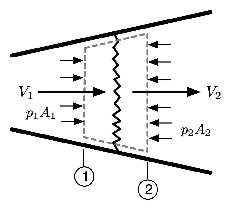
Control volume around shock — Figure 1:Control volume around a shock.

Figure 1 shows a control volume around a shock wave, in a duct with varying area. The thickness of the control volume is very small, on the order of the thickness of the shock itself (so $dx \sim 10^{-6}$ m). We will make the following assumptions about the flow:

steady, one-dimensional flow
adiabatic flow process: $\delta q = 0$ , and so $ds_e = 0$
no shaft work across the control volume: $\delta w_s = 0$
no potential change: $dz = 0$
constant area around the shock: $A_1 = A_2$

We can apply conservation of mass to this control volume:

\rho_1 A_1 V_1 = \rho_2 A_2 V_2

(129)

\rho_1 V_1 = \rho_2 V_2 \;,

(130)

conservation of energy:

\begin{gather*} h_{t1} + q = h_{t2} + w_s \\ h_{t1} = h_{t2} \end{gather*}

(131)

h_1 + \frac{V_1^2}{2} = h_2 + \frac{V_2^2}{2} \;,

(132)

and momentum:

\begin{gather*} \sum{F_x} = \dot{m} \left( V_{\text{out},x} - V_{\text{in}, x} \right) = \dot{m} \left( V_{2x} - V_{1x} \right) \\ p_1 A_1 - p_2 A_2 = ( p_1 - p_2 ) A = \dot{m} (V_2 - V_1) = \rho A V (V_2 - V_1) \\ p_1 - p_2 = (\rho V) V_2 - (\rho V) V_1 \\ p_1 - p_2 = \rho_2 V_2^2 - \rho_1 V_1^2 \end{gather*}

(133)

p_1 + \rho_1 V_1^2 = p_2 + \rho_2 V_2^2 \;.

(134)

For an arbitrary fluid, we have three equations: (130), (132), and (134). In a typical problem, we know the fluid and conditions before the shock, and want to find the conditions after the shock. Thus, our known variables are $\rho_1$ , $p_1$ , $h_1$ , and $V_1$ , while our unknown variables are $\rho_2$ , $p_2$ , $h_2$ , and $V_2$ . We need a fourth equation to close this system of equation: a property relation for the fluid, otherwise known as an equation of state.

Perfect gases¶

For ideal/perfect gases, we have the ideal gas equation of state, and can assume constant values for $c_p$ , $c_v$ , and $\gamma$ . We also have a convenient relationship for the speed of sound:

\begin{gather*} p = \rho R T \\ V = M a = M \sqrt{\gamma R T} \;. \end{gather*}

(135)

Incorporating these into Equation (130) we can obtain

\frac{p_1}{M_1}{\sqrt{T_1}} = \frac{p_2 M_2}{\sqrt{T_2}} \;.

(136)

With our stagnation relationship for temperature, $T_t = T \left( 1 + (\gamma-1)M^2 / 2 \right)^2$ , Equation (132) becomes

T_1 \left( 1 + \frac{\gamma-1}{2} M_1^2 \right) = T_2 \left( 1 + \frac{\gamma-1}{2} M_2^2 \right) \;,

(137)

which applies both around a normal shock and also at any point in a general flow with no work or heat transfer. Lastly, incorporating our relationships for perfect gases into Equation (134) we obtain

p_1 \left( 1 + \gamma M_1^2 \right) = p_2 \left( 1 + \gamma M_2^2 \right) \;.

(138)

Now, we have three equations and three unknowns: $M_2$ , $p_2$ , and $T_2$ . 😎

However, it is a bit of a pain to solve this complicated system of equations every time. Fortunately, we can combine all three together and eliminate pressure and temperature completely!

\left( \frac{1 + \gamma M_2^2}{1 + \gamma M_1^2} \right) \frac{M_1}{M_2} = \left( \frac{1 + \frac{\gamma-1}{2} M_2^2}{1 + \frac{\gamma-1}{2} M_1^2} \right)^{1/2} \;,

(139)

which can actually be solved to find $M_2 = f(\gamma, M_1)$ . A trivial solution to this equation is that $M_1 = M_2$ , where there is no shock. (What does this mean? Just that the governing equations we set up apply just fine for a flow where there is no shock—good news!)

For nontrivial solutions, with some painful algebra we can rearrange this equation into a recognizable form:

A \left( M_2^2 \right)^2 + B M_2^2 + C = 0 \;,

(140)

where $A, B, C = f(\gamma, M_1)$ . This looks like a quadratic equation! The only physically viable solution to this equation is

M_2^2 = \frac{M_1^2 + \frac{2}{\gamma-1}}{\frac{2 \gamma}{\gamma-1} M_1^2 - 1} \;.

(141)

gamma = 1.4
mach1 = np.linspace(1.0, 4.0, num=50, endpoint=True)
mach2 = np.sqrt((mach1**2 + 2/(gamma-1))/(2*gamma*mach1**2/(gamma-1) - 1))

plt.plot(mach1, mach2)
plt.xlabel(r'$M_1$')
plt.ylabel(r'$M_2$')
plt.title('Downstream Mach number versus upstream Mach number for normal shocks')
plt.grid(True)
plt.tight_layout()
plt.show()

Loading...

A typical problem flow is that we have $\gamma$ and $M_1$ , use these to determine $M_2$ , and then use Equations (137) and (138) to obtain $T_2$ and $p_2$ . More convenient versions of these equations are

\frac{T_2}{T_1} = \frac{1 + \frac{\gamma-1}{2} M_1^2}{1 + \frac{\gamma-1}{2} M_2^2}

(142)

\frac{p_2}{p_1} = \frac{1 + \gamma M_1^2}{1 + \gamma M_2^2} = \frac{2 \gamma M_1^2 - \gamma + 1}{\gamma + 1}

(143)

\frac{\rho_2}{\rho_1} = \frac{(\gamma+1) M_1^2}{(\gamma-1) M_1^2 + 2}

(144)