Review of thermodynamics¶

This module reviews the necessary thermodynamics concepts, including definitions, the laws of thermodynamics, and useful property relationships.

%matplotlib inline
from matplotlib import pyplot as plt

import numpy as np

# these lines are only for helping improve the display
import matplotlib_inline.backend_inline
matplotlib_inline.backend_inline.set_matplotlib_formats('pdf', 'png')
plt.rcParams['figure.dpi']= 300
plt.rcParams['savefig.dpi'] = 300
plt.rcParams['mathtext.fontset'] = 'cm'

Our study of gas dynamics will focus on a handful of important fluid properties:

density: $\rho = \frac{m}{V} = \frac{1}{\nu}$.
pressure: p = force/unit area. We work with absolute pressure (i.e., thermodynamic pressure), $p_{\text{abs}} = p_{\text{ambient}} + p_{\text{gage}}$.
temperature: T, which also must be absolute temperature.
viscosity: $\mu = \mu(T)$. Also kinematic viscosity: $\nu = \frac{\mu}{\rho}$.

Equations of state¶

For a fluid in general, the pressure, density, and temperature are not fully independent, and we can find one property given the other two. Equations of state describe the relationship between these properties, and are frequently expressed as $p = f(T, \rho)$. When dealing with liquids, we will frequently assume that they are incompressible and thus the density is constant.

For gases, we can frequently use the perfect, or ideal, gas equation of state:

\[ p = \rho R T \;, \]

where R is the specific gas constant:

\[ R = \frac{8314 \, \text{J}/\text{(kmol K)}}{MW} \]

and MW is the molecular weight of the gas. For air, R = 287 J/(kg K).

The ideal gas equation of state applies best for relatively low densities, or at relatively low pressures or high temperatures.

Thermodynamics definitions¶

Properties describe the state of a system.

intensive properties depend only on the state, and not how much stuff is in the system. Examples include temperature, density, and pressure
extensive properties depend on the amount of stuff (i.e., the mass) of the system. Examples include total internal energy (U) and volume (V)

We can also break down properties into type:

observable properties are directly measureable (p, T, V, mass)
mathematical properties come from combinations of other properties ($\rho$, $c_p$, h)
derived properties we arrive at from some analysis (internal energy from the First Law of thermodynamics, entropy from the Second Law)

Path/process: a series of consecutive states that define a unique journey from one state to another. Common features of processes that we will encounter or assume include:

adiabatic: no heat transfer ($\dot{Q} = 0$)
isothermal: constant temperature
isobaric: constant pressure
isentropic: constant entropy
isochoric: constant specific volume / density

Cycle: a sequence of processes that returns a system to its original state.

point function: a property, that depends only on the state of a system.

path function: not just a function of the state, but of the path/journey taken. Examples include heat and work.

Laws of Thermodynamics¶

$0^2$ Law¶

We may assume relations among properties (i.e., an equation of state) for a single component fluid, requiring only three independent properties to fix the state of the system. For a unit mass, we only need two independent properties: $p = f(\rho, T)$.

Zeroth Law¶

If two systems are connected by a nonadiabatic wall, their states will change until a new equilibrium state is reached. When they reach thermal equilibrium with each other, they have the same temperature.

Given two systems A and B that are in thermal equilibrium with each other, and if system B is also in thermal equilibrium with a third system C, then systems A and C are in thermal equilibrium with each other and share the same temperature.

(This is the law by which thermometers/thermocouples work.)

First Law of Thermodynamics¶

The 1st Law gives us conservation of energy. For a closed system,

\[ \sum Q = \sum W \;, \]

or the heat transfer into the system equals the work transfered from (i.e., done by) the system. So, for a process of a closed system:

\[\begin{gather*} Q = W + \Delta E \\ q = w + \Delta e \;, \end{gather*}\]

where E is total energy and e is the total energy per unit mass, defined as

\[ e \equiv u + \frac{V^2}{2} + gz + \text{others} \;, \]

where u is internal energy associated with molecular motion, $\frac{V^2}{2}$ is the kinetic energy, $gz$ is potential energy, and then other forms of energy may be considered.

For an infinitesimal process, conservation of energy is

\[ \delta q = \delta w + de \;, \]

where $\delta q$ and $\delta w$ are path functions, not exact differentials. For a stationary system, we can write this instead as

\[ \delta q = \delta w + du \;, \]

and in the case of reversible pressure work, we can represent work as $\delta w = p dv$. This leads to a useful form of conservation of energy:

\[ \delta q = p dv + du \;, \]

which leads to the derived property enthalpy: $h \equiv u + p v$. Differentiating that gives us

\[ dh = du + d(pv) = du + p dv + v dp \]

Internal energy and enthalpy also lead to the definitions of the specific heats:

\[\begin{gather*} c_p \equiv \left( \frac{\partial h}{\partial T} \right)_p \\ c_v \equiv \left( \frac{\partial u}{\partial T} \right)_v \;. \end{gather*}\]

Second Law of Thermodynamics¶

There are various versions/statements of the Second Law. The Kelvin—Planck version is:

It is impossible for an engine operating in a cycle to produce net work output when exchanging heat with only one temperature source.

tl;dr: the Second Law leads to the property of entropy and introduces the concept of degradation of energy quality through irreversible effects. Sources of these effects include friction, heat transfer from a finite temperature difference, and lack of pressure equilibrium. In other words, phenomena encountered in most realistic applications!

Under certain conditions we can assume a process is reversible, meaning that both the system and its surroundings can be restored to their original states. (However, in reality all processes are somewhat irreversible.)

It was observed that the integral of $\frac{\delta Q}{T}$ for a reversible process involving heat transfer is independent of the path taken during that process. If the change in some system quantity is independent of path, that means that this represents a change in a system property. Thus,

\[\begin{gather*} \Delta S \equiv \int \frac{\delta Q_R}{T} \\ ds \equiv \frac{\delta q_R}{T} \;, \end{gather*}\]

where the subscript R means that the heat transfer must be reversible, and S / s represents the property of entropy. We can use an exact differential with entropy (ds) because entropy is a system property, and changes in entropy depend only on the state of the system.

Property relations¶

We can combine the 1st and 2nd laws to come up with relationships between entropy and other properties.

Assuming a reversible process involving pressure-volume work, we can combine:

\[\begin{gather*} \delta q = \delta w + du \\ \delta w = p dv \\ \delta q = T ds \\ \rightarrow T ds = du + p dv \;. \end{gather*}\]

Similarly, we can take the differential of enthalpy and do a similar combination:

\[\begin{gather*} dh = du + p dv + v dp \\ \rightarrow T ds = dh - v dp = dh - \frac{dp}{\rho} \;. \end{gather*}\]

These thermodynamic relationships come from Gibbs identities.

Important: we assumed we were dealing with a reversible process (involving pressure-volume work) to get these expressions. However, these relations contain only properties — they are not path dependent! This means that they are valid for any end states of a system.

Perfect gases¶

If we are dealing with a perfect/ideal gas, we can simplify our expressions further. For an ideal gas, we know that

\[\begin{gather*} p = \rho R T \\ u = u (T) \\ c_v = \left( \frac{\partial u}{\partial T} \right)_v = \frac{du}{dT} \\ du = c_v dT \\ \rightarrow \Delta u = c_v \Delta T \end{gather*}\]

Similarly,

\[\begin{gather*} h = h(T) \\ c_p = \left( \frac{\partial h}{\partial T} \right)_p \\ \rightarrow \Delta h = c_p \Delta T \end{gather*}\]

If we assume or define as a reference state that internal energy and enthalpy are zero at absolute zero, i.e., $u(T=0) = 0$ and $h(T=0) = 0$, then we have that $u = c_v T$ and $h = c_p T$.

We can also define the specific heat ratio:

\[\begin{gather*} \gamma \equiv \frac{c_p}{c_v} \approx \begin{cases} 1.4 , \text{ diatomic gases (N$_2$, O$_2$, air)} \\ 1.7 , \text{ monotomic gases (He, Ar)} \end{cases} \end{gather*}\]

We also have relationships between the specific heats and the gas constant:

\[\begin{gather*} c_p - c_v = R \\ c_p = \frac{\gamma}{\gamma - 1} R \\ c_v = \frac{R}{\gamma - 1} \;. \end{gather*}\]

Entropy changes¶

By integrating the property relations for perfect gases, and taking advantage of our equation of state ($p = \rho R T$), we can get explicit equations for entropy change between two points in a process:

\[\begin{gather*} T ds = du + p dv \\ T ds = c_v dT + p dv \\ ds = c_v \frac{dT}{T} + \frac{p dv}{T} \;. \end{gather*}\]

Then, use the ideal gas equation of state:

\[ p = \rho R T \rightarrow p v = R T \rightarrow \frac{p}{T} = \frac{R}{v} \;. \]

\[\begin{gather*} ds = c_v \frac{dT}{T} + R \frac{dv}{v} \\ \Delta s_{1-2} = \int_{T_1}^{T_2} c_v (T) \frac{dT}{T} + R \int_{v_1}^{v_2} \frac{dv}{v} \;. \end{gather*}\]

Then, if we assume that specific heat is constant, $c_v(T) = c_v$, we can simplify further:

\[ \therefore \Delta s_{1-2} = c_v \ln \frac{T_2}{T_1} + R \ln \frac{v_2}{v_1} \]

Similarly, we can take that expression and obtain

\[\begin{gather*} \Delta s_{1-2} = c_p \ln \frac{v_2}{v_1} + c_v \ln \frac{p_2}{p_1} \\ \Delta s_{1-2} = c_p \ln \frac{T_2}{T_1} - R \ln \frac{p_2}{p_1} \end{gather*}\]

We can write functions to calculate the entropy change given initial and final values of temperature, volume, and pressure:

# Use properties of air
R = 287. # N*m/kg*K
c_v = 716.  # J/kg*K
c_p = 1000. # J/kg*K
gamma = c_p / c_v

# These functions can be used to calculate entropy given pairs
# of temperature, volume, and pressure.

def get_entropy_t_v(T1, T2, v1, v2):
    """Calculate entropy change given temperature and volume.
    """
    return c_v * np.log(T2 / T1) + R * np.log(v2 / v1)

def get_entropy_v_p(v1, v2, p2, p1):
    """Calculate entropy change given volume and pressure.
    """
    return c_p * np.log(v2 / v1) + c_v * np.log(p2 / p1)

def get_entropy_t_p(T1, T2, p1, p2):
    """Calculate entropy change given temperature and pressure.
    """
    return c_p * np.log(T2 / T1) - R * np.log(p2 / p1)

Polytropic processes¶

Polytropic processes follow the relation

\[ p v^n = \text{const} = C_1 \;, \]

where $n$ is the polytropic constant that depends on the specific process. With the ideal gas equation of state, we can also get relations with temperature:

\[\begin{gather*} T v^{n-1} = C_2 \\ T p^{\frac{1-n}{n}} = C_3 \;, \end{gather*}\]

where $C_1$, $C_2$, and $C_3$ are different constants.

Different values of $n$ correspond to different (polytropic) processes:

isobaric: $p = \text{const} \rightarrow n = 0$
isothermal: $T = \text{const} \rightarrow n = 1$
isentropic: $s = \text{const} \rightarrow n = \gamma$
isochoric: $v = \text{const} \rightarrow n = \infty$

Let’s visualize the $p-v$ diagrams for each of these processes:

# For a range of volumes, calculate pressure for various processes 
# using a given pressure-volume combination.

pressure_start = 5.0
volume_start = 2.0
volume_end = 8.0
volume = np.linspace(1.0, volume_end, num=100)

const_isobaric = pressure_start * volume_start**0
pressure_isobaric = const_isobaric / volume**0

const_isothermal = pressure_start * volume_start**1.0
pressure_isothermal = const_isothermal / volume**1.0

const_isentropic = pressure_start * volume_start**gamma
pressure_isentropic = const_isentropic / volume**gamma

# isochoric is a bit different
pressure_isochoric = np.linspace(
    np.min(pressure_isentropic), 
    np.max(pressure_isentropic), num=100
    )
volume_isochoric = np.ones_like(pressure_isochoric) * volume_start

# Now, plot everything:
plt.plot(volume, pressure_isobaric)
plt.text(volume_end*0.6, np.max(pressure_isobaric)*1.1, 
         r'$n = 0$', verticalalignment='bottom')
plt.plot(volume, pressure_isothermal)
plt.text(volume_end*0.6, np.min(pressure_isothermal)*2, 
         r'$n = 1$', verticalalignment='bottom')
plt.plot(volume, pressure_isentropic)
plt.text(volume_end*0.6, np.min(pressure_isentropic)*0.9, 
         r'$n = \gamma$', verticalalignment='top')
plt.plot(volume_isochoric, pressure_isochoric)
plt.text(volume_start*1.1, max(pressure_isochoric)*0.9, 
         r'$n = \infty$', horizontalalignment='left')
plt.xlabel('volume')
plt.ylabel('pressure')
plt.ylim(ymin=-0.5)
plt.tight_layout()
plt.show()

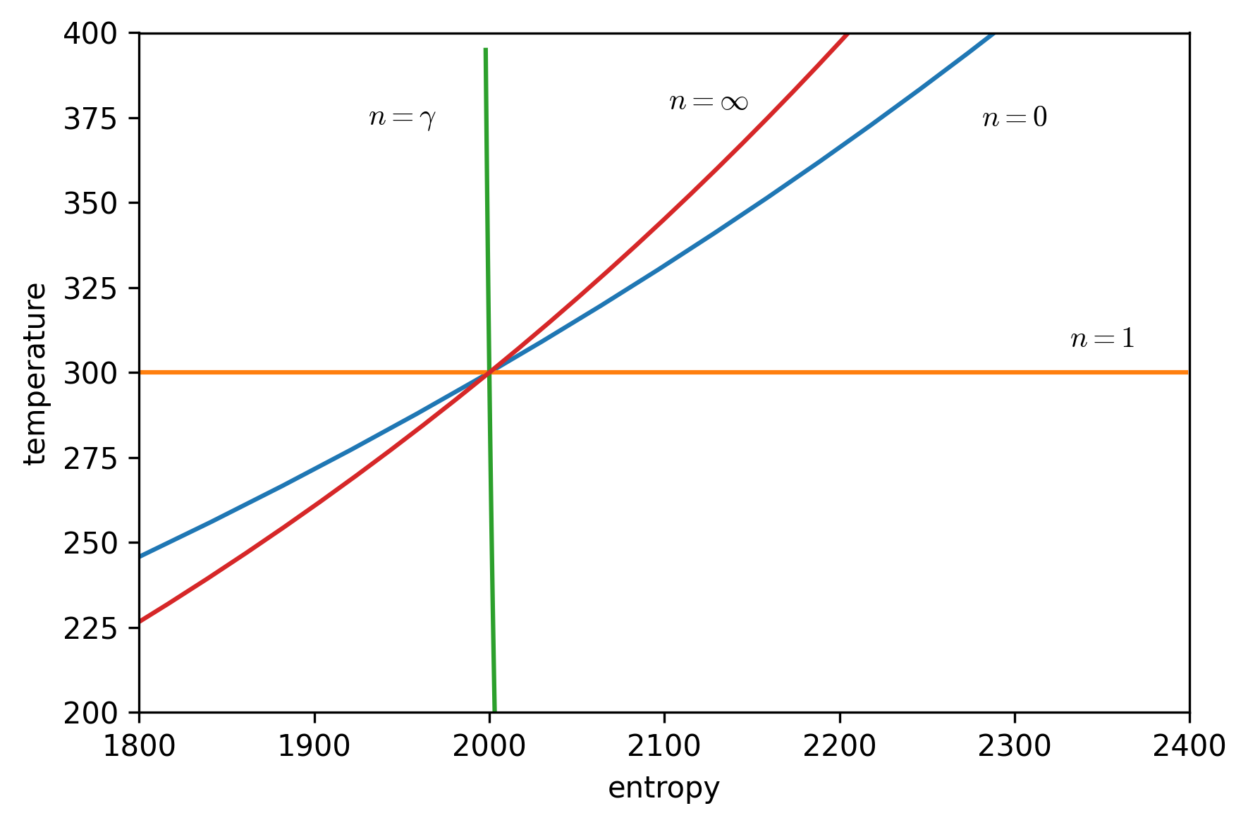
Using our relations for entropy changes, we can also visualize the $T-s$ diagrams for these processes:

temperature_start = 300
entropy_start = 2000

const_isobaric = temperature_start * volume_start**(-1)
temperature_isobaric = const_isobaric / volume**(-1)
entropy_isobaric = (
    entropy_start + 
    get_entropy_t_v(temperature_start, temperature_isobaric, volume_start, volume)
    )

temperature_isothermal = temperature_start * np.ones_like(volume)
entropy_isothermal = (
    entropy_start + 
    get_entropy_t_v(temperature_start, temperature_isothermal, volume_start, volume)
    )

# The limit of (1-n)/n as n-> infinity is -1
const_isochoric = temperature_start * pressure_start**(-1)
temperature_isochoric = const_isochoric / pressure_isochoric**(-1)
entropy_isochoric = (
    entropy_start + 
    get_entropy_t_p(temperature_start, temperature_isochoric, pressure_start, pressure_isochoric)
    )

# isentropic is a bit different
const_isentropic = temperature_start * volume_start**(gamma - 1)
temperature_isentropic = const_isentropic / volume**(gamma - 1)
entropy_isentropic = (
    entropy_start + 
    get_entropy_t_v(temperature_start, temperature_isentropic, volume_start, volume)
    )

# Now, plot everything:
plt.plot(entropy_isobaric, temperature_isobaric)
plt.text(2300, 375, r'$n = 0$', 
         verticalalignment='center', horizontalalignment='center'
         )
plt.plot(entropy_isothermal, temperature_isothermal)
plt.text(2350, 310, r'$n = 1$', 
         verticalalignment='center', horizontalalignment='center'
         )
plt.plot(entropy_isentropic, temperature_isentropic)
plt.text(1950, 375, r'$n = \gamma$', 
         verticalalignment='center', horizontalalignment='center'
         )
plt.plot(entropy_isochoric, temperature_isochoric)
plt.text(2125, 380, r'$n = \infty$', 
         verticalalignment='center', horizontalalignment='center'
         )
plt.xlabel('entropy')
plt.ylabel('temperature')
plt.axis([1800, 2400, 200, 400])
plt.tight_layout()
plt.show()

Gas Dynamics notes